Video classification with a 3D convolutional neural network

This tutorial demonstrates training a 3D convolutional neural network (CNN) for video classification using the UCF101 action recognition dataset. A 3D CNN uses a three-dimensional filter to perform convolutions. The kernel is able to slide in three directions, whereas in a 2D CNN it can slide in two dimensions. The model is based on the work published in A Closer Look at Spatiotemporal Convolutions for Action Recognition by D. Tran et al. (2017). In this tutorial, you will:

Build an input pipeline
Build a 3D convolutional neural network model with residual connections using Keras functional API
Train the model
Evaluate and test the model

This video classification tutorial is the second part in a series of TensorFlow video tutorials. Here are the other three tutorials:

Load video data: This tutorial explains much of the code used in this document.
MoViNet for streaming action recognition: Get familiar with the MoViNet models that are available on TF Hub.
Transfer learning for video classification with MoViNet: This tutorial explains how to use a pre-trained video classification model trained on a different dataset with the UCF-101 dataset.

Setup

Begin by installing and importing some necessary libraries, including: remotezip to inspect the contents of a ZIP file, tqdm to use a progress bar, OpenCV to process video files, einops for performing more complex tensor operations, and tensorflow_docs for embedding data in a Jupyter notebook.

pip install remotezip tqdm opencv-python einops
pip install -U tensorflow keras

import tqdm
import random
import pathlib
import itertools
import collections

import cv2
import einops
import numpy as np
import remotezip as rz
import seaborn as sns
import matplotlib.pyplot as plt

import tensorflow as tf
import keras
from keras import layers

2024-08-16 07:58:22.216693: E external/local_xla/xla/stream_executor/cuda/cuda_fft.cc:485] Unable to register cuFFT factory: Attempting to register factory for plugin cuFFT when one has already been registered
2024-08-16 07:58:22.237981: E external/local_xla/xla/stream_executor/cuda/cuda_dnn.cc:8454] Unable to register cuDNN factory: Attempting to register factory for plugin cuDNN when one has already been registered
2024-08-16 07:58:22.244520: E external/local_xla/xla/stream_executor/cuda/cuda_blas.cc:1452] Unable to register cuBLAS factory: Attempting to register factory for plugin cuBLAS when one has already been registered

Load and preprocess video data

The hidden cell below defines helper functions to download a slice of data from the UCF-101 dataset, and load it into a tf.data.Dataset. You can learn more about the specific preprocessing steps in the Loading video data tutorial, which walks you through this code in more detail.

The FrameGenerator class at the end of the hidden block is the most important utility here. It creates an iterable object that can feed data into the TensorFlow data pipeline. Specifically, this class contains a Python generator that loads the video frames along with its encoded label. The generator (__call__) function yields the frame array produced by frames_from_video_file and a one-hot encoded vector of the label associated with the set of frames.

def list_files_per_class(zip_url):
  """
    List the files in each class of the dataset given the zip URL.

    Args:
      zip_url: URL from which the files can be unzipped. 

    Return:
      files: List of files in each of the classes.
  """
  files = []
  with rz.RemoteZip(URL) as zip:
    for zip_info in zip.infolist():
      files.append(zip_info.filename)
  return files

def get_class(fname):
  """
    Retrieve the name of the class given a filename.

    Args:
      fname: Name of the file in the UCF101 dataset.

    Return:
      Class that the file belongs to.
  """
  return fname.split('_')[-3]

def get_files_per_class(files):
  """
    Retrieve the files that belong to each class. 

    Args:
      files: List of files in the dataset.

    Return:
      Dictionary of class names (key) and files (values).
  """
  files_for_class = collections.defaultdict(list)
  for fname in files:
    class_name = get_class(fname)
    files_for_class[class_name].append(fname)
  return files_for_class

def download_from_zip(zip_url, to_dir, file_names):
  """
    Download the contents of the zip file from the zip URL.

    Args:
      zip_url: Zip URL containing data.
      to_dir: Directory to download data to.
      file_names: Names of files to download.
  """
  with rz.RemoteZip(zip_url) as zip:
    for fn in tqdm.tqdm(file_names):
      class_name = get_class(fn)
      zip.extract(fn, str(to_dir / class_name))
      unzipped_file = to_dir / class_name / fn

      fn = pathlib.Path(fn).parts[-1]
      output_file = to_dir / class_name / fn
      unzipped_file.rename(output_file,)

def split_class_lists(files_for_class, count):
  """
    Returns the list of files belonging to a subset of data as well as the remainder of
    files that need to be downloaded.

    Args:
      files_for_class: Files belonging to a particular class of data.
      count: Number of files to download.

    Return:
      split_files: Files belonging to the subset of data.
      remainder: Dictionary of the remainder of files that need to be downloaded.
  """
  split_files = []
  remainder = {}
  for cls in files_for_class:
    split_files.extend(files_for_class[cls][:count])
    remainder[cls] = files_for_class[cls][count:]
  return split_files, remainder

def download_ufc_101_subset(zip_url, num_classes, splits, download_dir):
  """
    Download a subset of the UFC101 dataset and split them into various parts, such as
    training, validation, and test. 

    Args:
      zip_url: Zip URL containing data.
      num_classes: Number of labels.
      splits: Dictionary specifying the training, validation, test, etc. (key) division of data 
              (value is number of files per split).
      download_dir: Directory to download data to.

    Return:
      dir: Posix path of the resulting directories containing the splits of data.
  """
  files = list_files_per_class(zip_url)
  for f in files:
    tokens = f.split('/')
    if len(tokens) <= 2:
      files.remove(f) # Remove that item from the list if it does not have a filename

  files_for_class = get_files_per_class(files)

  classes = list(files_for_class.keys())[:num_classes]

  for cls in classes:
    new_files_for_class = files_for_class[cls]
    random.shuffle(new_files_for_class)
    files_for_class[cls] = new_files_for_class

  # Only use the number of classes you want in the dictionary
  files_for_class = {x: files_for_class[x] for x in list(files_for_class)[:num_classes]}

  dirs = {}
  for split_name, split_count in splits.items():
    print(split_name, ":")
    split_dir = download_dir / split_name
    split_files, files_for_class = split_class_lists(files_for_class, split_count)
    download_from_zip(zip_url, split_dir, split_files)
    dirs[split_name] = split_dir

  return dirs

def format_frames(frame, output_size):
  """
    Pad and resize an image from a video.

    Args:
      frame: Image that needs to resized and padded. 
      output_size: Pixel size of the output frame image.

    Return:
      Formatted frame with padding of specified output size.
  """
  frame = tf.image.convert_image_dtype(frame, tf.float32)
  frame = tf.image.resize_with_pad(frame, *output_size)
  return frame

def frames_from_video_file(video_path, n_frames, output_size = (224,224), frame_step = 15):
  """
    Creates frames from each video file present for each category.

    Args:
      video_path: File path to the video.
      n_frames: Number of frames to be created per video file.
      output_size: Pixel size of the output frame image.

    Return:
      An NumPy array of frames in the shape of (n_frames, height, width, channels).
  """
  # Read each video frame by frame
  result = []
  src = cv2.VideoCapture(str(video_path))  

  video_length = src.get(cv2.CAP_PROP_FRAME_COUNT)

  need_length = 1 + (n_frames - 1) * frame_step

  if need_length > video_length:
    start = 0
  else:
    max_start = video_length - need_length
    start = random.randint(0, max_start + 1)

  src.set(cv2.CAP_PROP_POS_FRAMES, start)
  # ret is a boolean indicating whether read was successful, frame is the image itself
  ret, frame = src.read()
  result.append(format_frames(frame, output_size))

  for _ in range(n_frames - 1):
    for _ in range(frame_step):
      ret, frame = src.read()
    if ret:
      frame = format_frames(frame, output_size)
      result.append(frame)
    else:
      result.append(np.zeros_like(result[0]))
  src.release()
  result = np.array(result)[..., [2, 1, 0]]

  return result

class FrameGenerator:
  def __init__(self, path, n_frames, training = False):
    """ Returns a set of frames with their associated label. 

      Args:
        path: Video file paths.
        n_frames: Number of frames. 
        training: Boolean to determine if training dataset is being created.
    """
    self.path = path
    self.n_frames = n_frames
    self.training = training
    self.class_names = sorted(set(p.name for p in self.path.iterdir() if p.is_dir()))
    self.class_ids_for_name = dict((name, idx) for idx, name in enumerate(self.class_names))

  def get_files_and_class_names(self):
    video_paths = list(self.path.glob('*/*.avi'))
    classes = [p.parent.name for p in video_paths] 
    return video_paths, classes

  def __call__(self):
    video_paths, classes = self.get_files_and_class_names()

    pairs = list(zip(video_paths, classes))

    if self.training:
      random.shuffle(pairs)

    for path, name in pairs:
      video_frames = frames_from_video_file(path, self.n_frames) 
      label = self.class_ids_for_name[name] # Encode labels
      yield video_frames, label

URL = 'https://storage.googleapis.com/thumos14_files/UCF101_videos.zip'
download_dir = pathlib.Path('./UCF101_subset/')
subset_paths = download_ufc_101_subset(URL, 
                        num_classes = 10, 
                        splits = {"train": 30, "val": 10, "test": 10},
                        download_dir = download_dir)

train :
100%|██████████| 300/300 [00:18<00:00, 15.82it/s]
val :
100%|██████████| 100/100 [00:06<00:00, 15.23it/s]
test :
100%|██████████| 100/100 [00:05<00:00, 19.10it/s]

Create the training, validation, and test sets (train_ds, val_ds, and test_ds).

n_frames = 10
batch_size = 8

output_signature = (tf.TensorSpec(shape = (None, None, None, 3), dtype = tf.float32),
                    tf.TensorSpec(shape = (), dtype = tf.int16))

train_ds = tf.data.Dataset.from_generator(FrameGenerator(subset_paths['train'], n_frames, training=True),
                                          output_signature = output_signature)


# Batch the data
train_ds = train_ds.batch(batch_size)

val_ds = tf.data.Dataset.from_generator(FrameGenerator(subset_paths['val'], n_frames),
                                        output_signature = output_signature)
val_ds = val_ds.batch(batch_size)

test_ds = tf.data.Dataset.from_generator(FrameGenerator(subset_paths['test'], n_frames),
                                         output_signature = output_signature)

test_ds = test_ds.batch(batch_size)

WARNING: All log messages before absl::InitializeLog() is called are written to STDERR
I0000 00:00:1723795136.342510  256222 cuda_executor.cc:1015] successful NUMA node read from SysFS had negative value (-1), but there must be at least one NUMA node, so returning NUMA node zero. See more at https://github.com/torvalds/linux/blob/v6.0/Documentation/ABI/testing/sysfs-bus-pci#L344-L355
I0000 00:00:1723795136.346466  256222 cuda_executor.cc:1015] successful NUMA node read from SysFS had negative value (-1), but there must be at least one NUMA node, so returning NUMA node zero. See more at https://github.com/torvalds/linux/blob/v6.0/Documentation/ABI/testing/sysfs-bus-pci#L344-L355
I0000 00:00:1723795136.350256  256222 cuda_executor.cc:1015] successful NUMA node read from SysFS had negative value (-1), but there must be at least one NUMA node, so returning NUMA node zero. See more at https://github.com/torvalds/linux/blob/v6.0/Documentation/ABI/testing/sysfs-bus-pci#L344-L355
I0000 00:00:1723795136.355717  256222 cuda_executor.cc:1015] successful NUMA node read from SysFS had negative value (-1), but there must be at least one NUMA node, so returning NUMA node zero. See more at https://github.com/torvalds/linux/blob/v6.0/Documentation/ABI/testing/sysfs-bus-pci#L344-L355
I0000 00:00:1723795136.367117  256222 cuda_executor.cc:1015] successful NUMA node read from SysFS had negative value (-1), but there must be at least one NUMA node, so returning NUMA node zero. See more at https://github.com/torvalds/linux/blob/v6.0/Documentation/ABI/testing/sysfs-bus-pci#L344-L355
I0000 00:00:1723795136.370661  256222 cuda_executor.cc:1015] successful NUMA node read from SysFS had negative value (-1), but there must be at least one NUMA node, so returning NUMA node zero. See more at https://github.com/torvalds/linux/blob/v6.0/Documentation/ABI/testing/sysfs-bus-pci#L344-L355
I0000 00:00:1723795136.376018  256222 cuda_executor.cc:1015] successful NUMA node read from SysFS had negative value (-1), but there must be at least one NUMA node, so returning NUMA node zero. See more at https://github.com/torvalds/linux/blob/v6.0/Documentation/ABI/testing/sysfs-bus-pci#L344-L355
I0000 00:00:1723795136.379583  256222 cuda_executor.cc:1015] successful NUMA node read from SysFS had negative value (-1), but there must be at least one NUMA node, so returning NUMA node zero. See more at https://github.com/torvalds/linux/blob/v6.0/Documentation/ABI/testing/sysfs-bus-pci#L344-L355
I0000 00:00:1723795136.383093  256222 cuda_executor.cc:1015] successful NUMA node read from SysFS had negative value (-1), but there must be at least one NUMA node, so returning NUMA node zero. See more at https://github.com/torvalds/linux/blob/v6.0/Documentation/ABI/testing/sysfs-bus-pci#L344-L355
I0000 00:00:1723795136.386591  256222 cuda_executor.cc:1015] successful NUMA node read from SysFS had negative value (-1), but there must be at least one NUMA node, so returning NUMA node zero. See more at https://github.com/torvalds/linux/blob/v6.0/Documentation/ABI/testing/sysfs-bus-pci#L344-L355
I0000 00:00:1723795136.390166  256222 cuda_executor.cc:1015] successful NUMA node read from SysFS had negative value (-1), but there must be at least one NUMA node, so returning NUMA node zero. See more at https://github.com/torvalds/linux/blob/v6.0/Documentation/ABI/testing/sysfs-bus-pci#L344-L355
I0000 00:00:1723795136.393648  256222 cuda_executor.cc:1015] successful NUMA node read from SysFS had negative value (-1), but there must be at least one NUMA node, so returning NUMA node zero. See more at https://github.com/torvalds/linux/blob/v6.0/Documentation/ABI/testing/sysfs-bus-pci#L344-L355
I0000 00:00:1723795137.619335  256222 cuda_executor.cc:1015] successful NUMA node read from SysFS had negative value (-1), but there must be at least one NUMA node, so returning NUMA node zero. See more at https://github.com/torvalds/linux/blob/v6.0/Documentation/ABI/testing/sysfs-bus-pci#L344-L355
I0000 00:00:1723795137.621400  256222 cuda_executor.cc:1015] successful NUMA node read from SysFS had negative value (-1), but there must be at least one NUMA node, so returning NUMA node zero. See more at https://github.com/torvalds/linux/blob/v6.0/Documentation/ABI/testing/sysfs-bus-pci#L344-L355
I0000 00:00:1723795137.623398  256222 cuda_executor.cc:1015] successful NUMA node read from SysFS had negative value (-1), but there must be at least one NUMA node, so returning NUMA node zero. See more at https://github.com/torvalds/linux/blob/v6.0/Documentation/ABI/testing/sysfs-bus-pci#L344-L355
I0000 00:00:1723795137.625485  256222 cuda_executor.cc:1015] successful NUMA node read from SysFS had negative value (-1), but there must be at least one NUMA node, so returning NUMA node zero. See more at https://github.com/torvalds/linux/blob/v6.0/Documentation/ABI/testing/sysfs-bus-pci#L344-L355
I0000 00:00:1723795137.627506  256222 cuda_executor.cc:1015] successful NUMA node read from SysFS had negative value (-1), but there must be at least one NUMA node, so returning NUMA node zero. See more at https://github.com/torvalds/linux/blob/v6.0/Documentation/ABI/testing/sysfs-bus-pci#L344-L355
I0000 00:00:1723795137.629390  256222 cuda_executor.cc:1015] successful NUMA node read from SysFS had negative value (-1), but there must be at least one NUMA node, so returning NUMA node zero. See more at https://github.com/torvalds/linux/blob/v6.0/Documentation/ABI/testing/sysfs-bus-pci#L344-L355
I0000 00:00:1723795137.631255  256222 cuda_executor.cc:1015] successful NUMA node read from SysFS had negative value (-1), but there must be at least one NUMA node, so returning NUMA node zero. See more at https://github.com/torvalds/linux/blob/v6.0/Documentation/ABI/testing/sysfs-bus-pci#L344-L355
I0000 00:00:1723795137.633243  256222 cuda_executor.cc:1015] successful NUMA node read from SysFS had negative value (-1), but there must be at least one NUMA node, so returning NUMA node zero. See more at https://github.com/torvalds/linux/blob/v6.0/Documentation/ABI/testing/sysfs-bus-pci#L344-L355
I0000 00:00:1723795137.635174  256222 cuda_executor.cc:1015] successful NUMA node read from SysFS had negative value (-1), but there must be at least one NUMA node, so returning NUMA node zero. See more at https://github.com/torvalds/linux/blob/v6.0/Documentation/ABI/testing/sysfs-bus-pci#L344-L355
I0000 00:00:1723795137.637074  256222 cuda_executor.cc:1015] successful NUMA node read from SysFS had negative value (-1), but there must be at least one NUMA node, so returning NUMA node zero. See more at https://github.com/torvalds/linux/blob/v6.0/Documentation/ABI/testing/sysfs-bus-pci#L344-L355
I0000 00:00:1723795137.638951  256222 cuda_executor.cc:1015] successful NUMA node read from SysFS had negative value (-1), but there must be at least one NUMA node, so returning NUMA node zero. See more at https://github.com/torvalds/linux/blob/v6.0/Documentation/ABI/testing/sysfs-bus-pci#L344-L355
I0000 00:00:1723795137.640940  256222 cuda_executor.cc:1015] successful NUMA node read from SysFS had negative value (-1), but there must be at least one NUMA node, so returning NUMA node zero. See more at https://github.com/torvalds/linux/blob/v6.0/Documentation/ABI/testing/sysfs-bus-pci#L344-L355
I0000 00:00:1723795137.679357  256222 cuda_executor.cc:1015] successful NUMA node read from SysFS had negative value (-1), but there must be at least one NUMA node, so returning NUMA node zero. See more at https://github.com/torvalds/linux/blob/v6.0/Documentation/ABI/testing/sysfs-bus-pci#L344-L355
I0000 00:00:1723795137.681337  256222 cuda_executor.cc:1015] successful NUMA node read from SysFS had negative value (-1), but there must be at least one NUMA node, so returning NUMA node zero. See more at https://github.com/torvalds/linux/blob/v6.0/Documentation/ABI/testing/sysfs-bus-pci#L344-L355
I0000 00:00:1723795137.683257  256222 cuda_executor.cc:1015] successful NUMA node read from SysFS had negative value (-1), but there must be at least one NUMA node, so returning NUMA node zero. See more at https://github.com/torvalds/linux/blob/v6.0/Documentation/ABI/testing/sysfs-bus-pci#L344-L355
I0000 00:00:1723795137.685319  256222 cuda_executor.cc:1015] successful NUMA node read from SysFS had negative value (-1), but there must be at least one NUMA node, so returning NUMA node zero. See more at https://github.com/torvalds/linux/blob/v6.0/Documentation/ABI/testing/sysfs-bus-pci#L344-L355
I0000 00:00:1723795137.687152  256222 cuda_executor.cc:1015] successful NUMA node read from SysFS had negative value (-1), but there must be at least one NUMA node, so returning NUMA node zero. See more at https://github.com/torvalds/linux/blob/v6.0/Documentation/ABI/testing/sysfs-bus-pci#L344-L355
I0000 00:00:1723795137.689047  256222 cuda_executor.cc:1015] successful NUMA node read from SysFS had negative value (-1), but there must be at least one NUMA node, so returning NUMA node zero. See more at https://github.com/torvalds/linux/blob/v6.0/Documentation/ABI/testing/sysfs-bus-pci#L344-L355
I0000 00:00:1723795137.690916  256222 cuda_executor.cc:1015] successful NUMA node read from SysFS had negative value (-1), but there must be at least one NUMA node, so returning NUMA node zero. See more at https://github.com/torvalds/linux/blob/v6.0/Documentation/ABI/testing/sysfs-bus-pci#L344-L355
I0000 00:00:1723795137.692935  256222 cuda_executor.cc:1015] successful NUMA node read from SysFS had negative value (-1), but there must be at least one NUMA node, so returning NUMA node zero. See more at https://github.com/torvalds/linux/blob/v6.0/Documentation/ABI/testing/sysfs-bus-pci#L344-L355
I0000 00:00:1723795137.694785  256222 cuda_executor.cc:1015] successful NUMA node read from SysFS had negative value (-1), but there must be at least one NUMA node, so returning NUMA node zero. See more at https://github.com/torvalds/linux/blob/v6.0/Documentation/ABI/testing/sysfs-bus-pci#L344-L355
I0000 00:00:1723795137.697120  256222 cuda_executor.cc:1015] successful NUMA node read from SysFS had negative value (-1), but there must be at least one NUMA node, so returning NUMA node zero. See more at https://github.com/torvalds/linux/blob/v6.0/Documentation/ABI/testing/sysfs-bus-pci#L344-L355
I0000 00:00:1723795137.699500  256222 cuda_executor.cc:1015] successful NUMA node read from SysFS had negative value (-1), but there must be at least one NUMA node, so returning NUMA node zero. See more at https://github.com/torvalds/linux/blob/v6.0/Documentation/ABI/testing/sysfs-bus-pci#L344-L355
I0000 00:00:1723795137.701941  256222 cuda_executor.cc:1015] successful NUMA node read from SysFS had negative value (-1), but there must be at least one NUMA node, so returning NUMA node zero. See more at https://github.com/torvalds/linux/blob/v6.0/Documentation/ABI/testing/sysfs-bus-pci#L344-L355

Create the model

The following 3D convolutional neural network model is based off the paper A Closer Look at Spatiotemporal Convolutions for Action Recognition by D. Tran et al. (2017). The paper compares several versions of 3D ResNets. Instead of operating on a single image with dimensions (height, width), like standard ResNets, these operate on video volume (time, height, width). The most obvious approach to this problem would be replace each 2D convolution (layers.Conv2D) with a 3D convolution (layers.Conv3D).

This tutorial uses a (2 + 1)D convolution with residual connections. The (2 + 1)D convolution allows for the decomposition of the spatial and temporal dimensions, therefore creating two separate steps. An advantage of this approach is that factorizing the convolutions into spatial and temporal dimensions saves parameters.

For each output location a 3D convolution combines all the vectors from a 3D patch of the volume to create one vector in the output volume.

3D convolutions

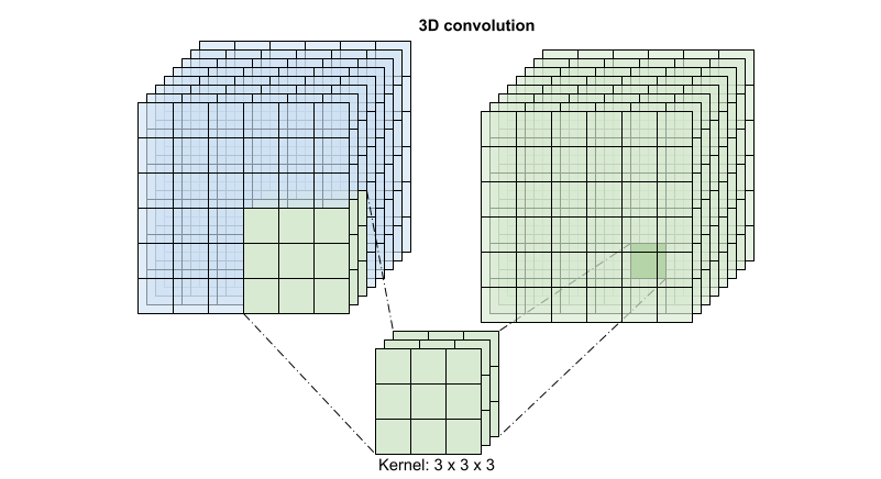
This operation is takes time * height * width * channels inputs and produces channels outputs (assuming the number of input and output channels are the same. So a 3D convolution layer with a kernel size of (3 x 3 x 3) would need a weight-matrix with 27 * channels ** 2 entries. The reference paper found that a more effective & efficient approach was to factorize the convolution. Instead of a single 3D convolution to process the time and space dimensions, they proposed a "(2+1)D" convolution which processes the space and time dimensions separately. The figure below shows the factored spatial and temporal convolutions of a (2 + 1)D convolution.

(2+1)D convolutions

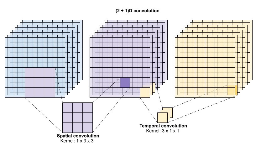
The main advantage of this approach is that it reduces the number of parameters. In the (2 + 1)D convolution the spatial convolution takes in data of the shape (1, width, height), while the temporal convolution takes in data of the shape (time, 1, 1). For example, a (2 + 1)D convolution with kernel size (3 x 3 x 3) would need weight matrices of size (9 * channels**2) + (3 * channels**2), less than half as many as the full 3D convolution. This tutorial implements (2 + 1)D ResNet18, where each convolution in the resnet is replaced by a (2+1)D convolution.

# Define the dimensions of one frame in the set of frames created
HEIGHT = 224
WIDTH = 224

class Conv2Plus1D(keras.layers.Layer):
  def __init__(self, filters, kernel_size, padding):
    """
      A sequence of convolutional layers that first apply the convolution operation over the
      spatial dimensions, and then the temporal dimension. 
    """
    super().__init__()
    self.seq = keras.Sequential([  
        # Spatial decomposition
        layers.Conv3D(filters=filters,
                      kernel_size=(1, kernel_size[1], kernel_size[2]),
                      padding=padding),
        # Temporal decomposition
        layers.Conv3D(filters=filters, 
                      kernel_size=(kernel_size[0], 1, 1),
                      padding=padding)
        ])

  def call(self, x):
    return self.seq(x)

A ResNet model is made from a sequence of residual blocks. A residual block has two branches. The main branch performs the calculation, but is difficult for gradients to flow through. The residual branch bypasses the main calculation and mostly just adds the input to the output of the main branch. Gradients flow easily through this branch. Therefore, an easy path from the loss function to any of the residual block's main branch will be present. This avoids the vanishing gradient problem.

Create the main branch of the residual block with the following class. In contrast to the standard ResNet structure this uses the custom Conv2Plus1D layer instead of layers.Conv2D.

class ResidualMain(keras.layers.Layer):
  """
    Residual block of the model with convolution, layer normalization, and the
    activation function, ReLU.
  """
  def __init__(self, filters, kernel_size):
    super().__init__()
    self.seq = keras.Sequential([
        Conv2Plus1D(filters=filters,
                    kernel_size=kernel_size,
                    padding='same'),
        layers.LayerNormalization(),
        layers.ReLU(),
        Conv2Plus1D(filters=filters, 
                    kernel_size=kernel_size,
                    padding='same'),
        layers.LayerNormalization()
    ])

  def call(self, x):
    return self.seq(x)

To add the residual branch to the main branch it needs to have the same size. The Project layer below deals with cases where the number of channels is changed on the branch. In particular, a sequence of densely-connected layer followed by normalization is added.

class Project(keras.layers.Layer):
  """
    Project certain dimensions of the tensor as the data is passed through different 
    sized filters and downsampled. 
  """
  def __init__(self, units):
    super().__init__()
    self.seq = keras.Sequential([
        layers.Dense(units),
        layers.LayerNormalization()
    ])

  def call(self, x):
    return self.seq(x)

Use add_residual_block to introduce a skip connection between the layers of the model.

def add_residual_block(input, filters, kernel_size):
  """
    Add residual blocks to the model. If the last dimensions of the input data
    and filter size does not match, project it such that last dimension matches.
  """
  out = ResidualMain(filters, 
                     kernel_size)(input)

  res = input
  # Using the Keras functional APIs, project the last dimension of the tensor to
  # match the new filter size
  if out.shape[-1] != input.shape[-1]:
    res = Project(out.shape[-1])(res)

  return layers.add([res, out])

Resizing the video is necessary to perform downsampling of the data. In particular, downsampling the video frames allow for the model to examine specific parts of frames to detect patterns that may be specific to a certain action. Through downsampling, non-essential information can be discarded. Moreoever, resizing the video will allow for dimensionality reduction and therefore faster processing through the model.

class ResizeVideo(keras.layers.Layer):
  def __init__(self, height, width):
    super().__init__()
    self.height = height
    self.width = width
    self.resizing_layer = layers.Resizing(self.height, self.width)

  def call(self, video):
    """
      Use the einops library to resize the tensor.  

      Args:
        video: Tensor representation of the video, in the form of a set of frames.

      Return:
        A downsampled size of the video according to the new height and width it should be resized to.
    """
    # b stands for batch size, t stands for time, h stands for height, 
    # w stands for width, and c stands for the number of channels.
    old_shape = einops.parse_shape(video, 'b t h w c')
    images = einops.rearrange(video, 'b t h w c -> (b t) h w c')
    images = self.resizing_layer(images)
    videos = einops.rearrange(
        images, '(b t) h w c -> b t h w c',
        t = old_shape['t'])
    return videos

Use the Keras functional API to build the residual network.

input_shape = (None, 10, HEIGHT, WIDTH, 3)
input = layers.Input(shape=(input_shape[1:]))
x = input

x = Conv2Plus1D(filters=16, kernel_size=(3, 7, 7), padding='same')(x)
x = layers.BatchNormalization()(x)
x = layers.ReLU()(x)
x = ResizeVideo(HEIGHT // 2, WIDTH // 2)(x)

# Block 1
x = add_residual_block(x, 16, (3, 3, 3))
x = ResizeVideo(HEIGHT // 4, WIDTH // 4)(x)

# Block 2
x = add_residual_block(x, 32, (3, 3, 3))
x = ResizeVideo(HEIGHT // 8, WIDTH // 8)(x)

# Block 3
x = add_residual_block(x, 64, (3, 3, 3))
x = ResizeVideo(HEIGHT // 16, WIDTH // 16)(x)

# Block 4
x = add_residual_block(x, 128, (3, 3, 3))

x = layers.GlobalAveragePooling3D()(x)
x = layers.Flatten()(x)
x = layers.Dense(10)(x)

model = keras.Model(input, x)

frames, label = next(iter(train_ds))
model.build(frames)

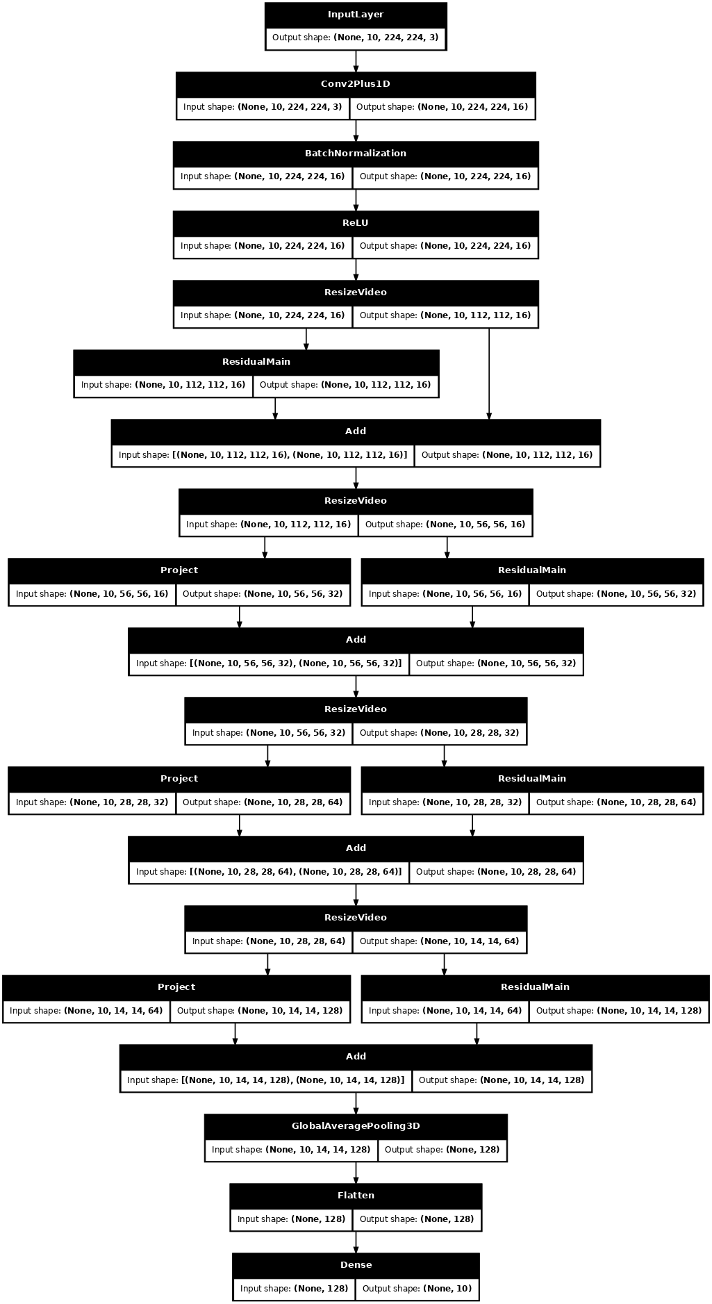
# Visualize the model
keras.utils.plot_model(model, expand_nested=True, dpi=60, show_shapes=True)

png

Train the model

For this tutorial, choose the tf.keras.optimizers.Adam optimizer and the tf.keras.losses.SparseCategoricalCrossentropy loss function. Use the metrics argument to the view the accuracy of the model performance at every step.

model.compile(loss = keras.losses.SparseCategoricalCrossentropy(from_logits=True), 
              optimizer = keras.optimizers.Adam(learning_rate = 0.0001), 
              metrics = ['accuracy'])

Train the model for 50 epoches with the Keras Model.fit method.

history = model.fit(x = train_ds,
                    epochs = 50, 
                    validation_data = val_ds)

Epoch 1/50
WARNING: All log messages before absl::InitializeLog() is called are written to STDERR
I0000 00:00:1723795151.433190  256397 service.cc:146] XLA service 0x7f870c033450 initialized for platform CUDA (this does not guarantee that XLA will be used). Devices:
I0000 00:00:1723795151.433225  256397 service.cc:154]   StreamExecutor device (0): Tesla T4, Compute Capability 7.5
I0000 00:00:1723795151.433229  256397 service.cc:154]   StreamExecutor device (1): Tesla T4, Compute Capability 7.5
I0000 00:00:1723795151.433232  256397 service.cc:154]   StreamExecutor device (2): Tesla T4, Compute Capability 7.5
I0000 00:00:1723795151.433235  256397 service.cc:154]   StreamExecutor device (3): Tesla T4, Compute Capability 7.5
I0000 00:00:1723795169.934874  256397 device_compiler.h:188] Compiled cluster using XLA!  This line is logged at most once for the lifetime of the process.
38/Unknown 81s 1s/step - accuracy: 0.1341 - loss: 2.5066
/usr/lib/python3.9/contextlib.py:137: UserWarning: Your input ran out of data; interrupting training. Make sure that your dataset or generator can generate at least `steps_per_epoch * epochs` batches. You may need to use the `.repeat()` function when building your dataset.
  self.gen.throw(typ, value, traceback)
38/38 ━━━━━━━━━━━━━━━━━━━━ 96s 2s/step - accuracy: 0.1350 - loss: 2.5029 - val_accuracy: 0.1700 - val_loss: 2.4099
Epoch 2/50
38/38 ━━━━━━━━━━━━━━━━━━━━ 49s 1s/step - accuracy: 0.2155 - loss: 2.1272 - val_accuracy: 0.2100 - val_loss: 2.1292
Epoch 3/50
38/38 ━━━━━━━━━━━━━━━━━━━━ 49s 1s/step - accuracy: 0.2407 - loss: 2.0321 - val_accuracy: 0.1800 - val_loss: 2.1674
Epoch 4/50
38/38 ━━━━━━━━━━━━━━━━━━━━ 50s 1s/step - accuracy: 0.3320 - loss: 1.8774 - val_accuracy: 0.2200 - val_loss: 2.1371
Epoch 5/50
38/38 ━━━━━━━━━━━━━━━━━━━━ 50s 1s/step - accuracy: 0.3561 - loss: 1.8134 - val_accuracy: 0.1700 - val_loss: 2.5758
Epoch 6/50
38/38 ━━━━━━━━━━━━━━━━━━━━ 50s 1s/step - accuracy: 0.3421 - loss: 1.7778 - val_accuracy: 0.2000 - val_loss: 2.4542
Epoch 7/50
38/38 ━━━━━━━━━━━━━━━━━━━━ 50s 1s/step - accuracy: 0.4468 - loss: 1.5379 - val_accuracy: 0.3100 - val_loss: 2.3473
Epoch 8/50
38/38 ━━━━━━━━━━━━━━━━━━━━ 50s 1s/step - accuracy: 0.4152 - loss: 1.5421 - val_accuracy: 0.3700 - val_loss: 1.8979
Epoch 9/50
38/38 ━━━━━━━━━━━━━━━━━━━━ 50s 1s/step - accuracy: 0.4987 - loss: 1.4076 - val_accuracy: 0.3300 - val_loss: 2.0729
Epoch 10/50
38/38 ━━━━━━━━━━━━━━━━━━━━ 50s 1s/step - accuracy: 0.4830 - loss: 1.4727 - val_accuracy: 0.4400 - val_loss: 1.9701
Epoch 11/50
38/38 ━━━━━━━━━━━━━━━━━━━━ 50s 1s/step - accuracy: 0.5045 - loss: 1.4261 - val_accuracy: 0.3500 - val_loss: 1.8626
Epoch 12/50
38/38 ━━━━━━━━━━━━━━━━━━━━ 50s 1s/step - accuracy: 0.5948 - loss: 1.2100 - val_accuracy: 0.4700 - val_loss: 1.6501
Epoch 13/50
38/38 ━━━━━━━━━━━━━━━━━━━━ 50s 1s/step - accuracy: 0.6074 - loss: 1.2345 - val_accuracy: 0.5700 - val_loss: 1.3051
Epoch 14/50
38/38 ━━━━━━━━━━━━━━━━━━━━ 50s 1s/step - accuracy: 0.6095 - loss: 1.0378 - val_accuracy: 0.4800 - val_loss: 1.4512
Epoch 15/50
38/38 ━━━━━━━━━━━━━━━━━━━━ 50s 1s/step - accuracy: 0.5720 - loss: 1.0935 - val_accuracy: 0.6200 - val_loss: 1.1746
Epoch 16/50
38/38 ━━━━━━━━━━━━━━━━━━━━ 50s 1s/step - accuracy: 0.6414 - loss: 1.0612 - val_accuracy: 0.5900 - val_loss: 1.1096
Epoch 17/50
38/38 ━━━━━━━━━━━━━━━━━━━━ 50s 1s/step - accuracy: 0.6466 - loss: 1.0072 - val_accuracy: 0.3400 - val_loss: 1.9732
Epoch 18/50
38/38 ━━━━━━━━━━━━━━━━━━━━ 50s 1s/step - accuracy: 0.6491 - loss: 1.0926 - val_accuracy: 0.5600 - val_loss: 1.0943
Epoch 19/50
38/38 ━━━━━━━━━━━━━━━━━━━━ 50s 1s/step - accuracy: 0.7055 - loss: 0.9202 - val_accuracy: 0.6800 - val_loss: 1.0248
Epoch 20/50
38/38 ━━━━━━━━━━━━━━━━━━━━ 50s 1s/step - accuracy: 0.7047 - loss: 0.8617 - val_accuracy: 0.6200 - val_loss: 0.9955
Epoch 21/50
38/38 ━━━━━━━━━━━━━━━━━━━━ 50s 1s/step - accuracy: 0.6403 - loss: 0.9750 - val_accuracy: 0.6600 - val_loss: 0.9456
Epoch 22/50
38/38 ━━━━━━━━━━━━━━━━━━━━ 50s 1s/step - accuracy: 0.7257 - loss: 0.8546 - val_accuracy: 0.4900 - val_loss: 1.4771
Epoch 23/50
38/38 ━━━━━━━━━━━━━━━━━━━━ 50s 1s/step - accuracy: 0.6771 - loss: 0.8721 - val_accuracy: 0.5800 - val_loss: 1.0957
Epoch 24/50
38/38 ━━━━━━━━━━━━━━━━━━━━ 50s 1s/step - accuracy: 0.7084 - loss: 0.8281 - val_accuracy: 0.6800 - val_loss: 0.9744
Epoch 25/50
38/38 ━━━━━━━━━━━━━━━━━━━━ 50s 1s/step - accuracy: 0.7980 - loss: 0.6998 - val_accuracy: 0.5100 - val_loss: 1.6530
Epoch 26/50
38/38 ━━━━━━━━━━━━━━━━━━━━ 50s 1s/step - accuracy: 0.6360 - loss: 0.9005 - val_accuracy: 0.5700 - val_loss: 1.2295
Epoch 27/50
38/38 ━━━━━━━━━━━━━━━━━━━━ 50s 1s/step - accuracy: 0.7020 - loss: 0.7782 - val_accuracy: 0.6000 - val_loss: 1.0399
Epoch 28/50
38/38 ━━━━━━━━━━━━━━━━━━━━ 50s 1s/step - accuracy: 0.6859 - loss: 0.8315 - val_accuracy: 0.6500 - val_loss: 0.9905
Epoch 29/50
38/38 ━━━━━━━━━━━━━━━━━━━━ 50s 1s/step - accuracy: 0.7159 - loss: 0.7938 - val_accuracy: 0.6800 - val_loss: 0.8693
Epoch 30/50
38/38 ━━━━━━━━━━━━━━━━━━━━ 50s 1s/step - accuracy: 0.7675 - loss: 0.6411 - val_accuracy: 0.6500 - val_loss: 0.9730
Epoch 31/50
38/38 ━━━━━━━━━━━━━━━━━━━━ 50s 1s/step - accuracy: 0.7884 - loss: 0.6418 - val_accuracy: 0.4800 - val_loss: 1.3806
Epoch 32/50
38/38 ━━━━━━━━━━━━━━━━━━━━ 50s 1s/step - accuracy: 0.7048 - loss: 0.7944 - val_accuracy: 0.6200 - val_loss: 0.9962
Epoch 33/50
38/38 ━━━━━━━━━━━━━━━━━━━━ 50s 1s/step - accuracy: 0.8176 - loss: 0.5833 - val_accuracy: 0.6700 - val_loss: 0.9532
Epoch 34/50
38/38 ━━━━━━━━━━━━━━━━━━━━ 50s 1s/step - accuracy: 0.7391 - loss: 0.6760 - val_accuracy: 0.7000 - val_loss: 0.9689
Epoch 35/50
38/38 ━━━━━━━━━━━━━━━━━━━━ 50s 1s/step - accuracy: 0.8041 - loss: 0.6246 - val_accuracy: 0.5900 - val_loss: 1.0407
Epoch 36/50
38/38 ━━━━━━━━━━━━━━━━━━━━ 50s 1s/step - accuracy: 0.7267 - loss: 0.6603 - val_accuracy: 0.5700 - val_loss: 1.1837
Epoch 37/50
38/38 ━━━━━━━━━━━━━━━━━━━━ 49s 1s/step - accuracy: 0.7862 - loss: 0.6348 - val_accuracy: 0.6400 - val_loss: 1.0391
Epoch 38/50
38/38 ━━━━━━━━━━━━━━━━━━━━ 49s 1s/step - accuracy: 0.7899 - loss: 0.6000 - val_accuracy: 0.6700 - val_loss: 0.8552
Epoch 39/50
38/38 ━━━━━━━━━━━━━━━━━━━━ 50s 1s/step - accuracy: 0.8233 - loss: 0.5389 - val_accuracy: 0.6800 - val_loss: 0.9595
Epoch 40/50
38/38 ━━━━━━━━━━━━━━━━━━━━ 49s 1s/step - accuracy: 0.8382 - loss: 0.5075 - val_accuracy: 0.7200 - val_loss: 0.7749
Epoch 41/50
38/38 ━━━━━━━━━━━━━━━━━━━━ 50s 1s/step - accuracy: 0.8411 - loss: 0.5221 - val_accuracy: 0.6800 - val_loss: 0.8257
Epoch 42/50
38/38 ━━━━━━━━━━━━━━━━━━━━ 50s 1s/step - accuracy: 0.8351 - loss: 0.4983 - val_accuracy: 0.6700 - val_loss: 0.9425
Epoch 43/50
38/38 ━━━━━━━━━━━━━━━━━━━━ 50s 1s/step - accuracy: 0.7883 - loss: 0.5487 - val_accuracy: 0.5800 - val_loss: 1.1208
Epoch 44/50
38/38 ━━━━━━━━━━━━━━━━━━━━ 50s 1s/step - accuracy: 0.7620 - loss: 0.6305 - val_accuracy: 0.7100 - val_loss: 0.8008
Epoch 45/50
38/38 ━━━━━━━━━━━━━━━━━━━━ 50s 1s/step - accuracy: 0.8250 - loss: 0.5602 - val_accuracy: 0.7000 - val_loss: 0.8332
Epoch 46/50
38/38 ━━━━━━━━━━━━━━━━━━━━ 49s 1s/step - accuracy: 0.8172 - loss: 0.5205 - val_accuracy: 0.6600 - val_loss: 0.9206
Epoch 47/50
38/38 ━━━━━━━━━━━━━━━━━━━━ 50s 1s/step - accuracy: 0.8438 - loss: 0.4675 - val_accuracy: 0.6800 - val_loss: 0.9416
Epoch 48/50
38/38 ━━━━━━━━━━━━━━━━━━━━ 50s 1s/step - accuracy: 0.7677 - loss: 0.8618 - val_accuracy: 0.5400 - val_loss: 1.5664
Epoch 49/50
38/38 ━━━━━━━━━━━━━━━━━━━━ 50s 1s/step - accuracy: 0.8111 - loss: 0.5301 - val_accuracy: 0.7400 - val_loss: 0.8227
Epoch 50/50
38/38 ━━━━━━━━━━━━━━━━━━━━ 50s 1s/step - accuracy: 0.8454 - loss: 0.4606 - val_accuracy: 0.7000 - val_loss: 0.9533

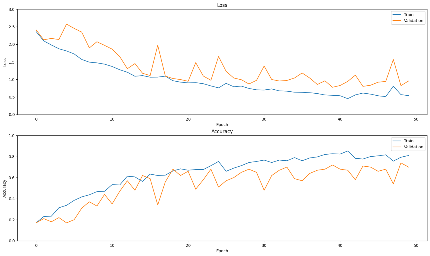
Visualize the results

Create plots of the loss and accuracy on the training and validation sets:

def plot_history(history):
  """
    Plotting training and validation learning curves.

    Args:
      history: model history with all the metric measures
  """
  fig, (ax1, ax2) = plt.subplots(2)

  fig.set_size_inches(18.5, 10.5)

  # Plot loss
  ax1.set_title('Loss')
  ax1.plot(history.history['loss'], label = 'train')
  ax1.plot(history.history['val_loss'], label = 'test')
  ax1.set_ylabel('Loss')

  # Determine upper bound of y-axis
  max_loss = max(history.history['loss'] + history.history['val_loss'])

  ax1.set_ylim([0, np.ceil(max_loss)])
  ax1.set_xlabel('Epoch')
  ax1.legend(['Train', 'Validation']) 

  # Plot accuracy
  ax2.set_title('Accuracy')
  ax2.plot(history.history['accuracy'],  label = 'train')
  ax2.plot(history.history['val_accuracy'], label = 'test')
  ax2.set_ylabel('Accuracy')
  ax2.set_ylim([0, 1])
  ax2.set_xlabel('Epoch')
  ax2.legend(['Train', 'Validation'])

  plt.show()

plot_history(history)

png

Evaluate the model

Use Keras Model.evaluate to get the loss and accuracy on the test dataset.

model.evaluate(test_ds, return_dict=True)

13/13 ━━━━━━━━━━━━━━━━━━━━ 11s 838ms/step - accuracy: 0.7469 - loss: 0.8416
{'accuracy': 0.6899999976158142, 'loss': 1.0032306909561157}

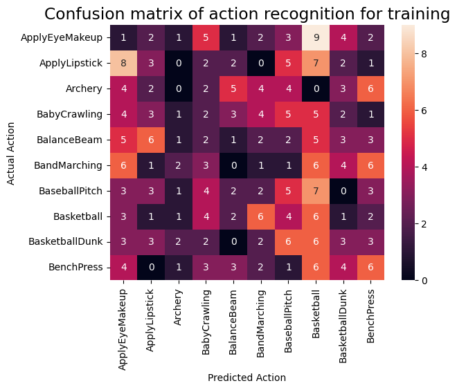
To visualize model performance further, use a confusion matrix. The confusion matrix allows you to assess the performance of the classification model beyond accuracy. In order to build the confusion matrix for this multi-class classification problem, get the actual values in the test set and the predicted values.

def get_actual_predicted_labels(dataset): 
  """
    Create a list of actual ground truth values and the predictions from the model.

    Args:
      dataset: An iterable data structure, such as a TensorFlow Dataset, with features and labels.

    Return:
      Ground truth and predicted values for a particular dataset.
  """
  actual = [labels for _, labels in dataset.unbatch()]
  predicted = model.predict(dataset)

  actual = tf.stack(actual, axis=0)
  predicted = tf.concat(predicted, axis=0)
  predicted = tf.argmax(predicted, axis=1)

  return actual, predicted

def plot_confusion_matrix(actual, predicted, labels, ds_type):
  cm = tf.math.confusion_matrix(actual, predicted)
  ax = sns.heatmap(cm, annot=True, fmt='g')
  sns.set(rc={'figure.figsize':(12, 12)})
  sns.set(font_scale=1.4)
  ax.set_title('Confusion matrix of action recognition for ' + ds_type)
  ax.set_xlabel('Predicted Action')
  ax.set_ylabel('Actual Action')
  plt.xticks(rotation=90)
  plt.yticks(rotation=0)
  ax.xaxis.set_ticklabels(labels)
  ax.yaxis.set_ticklabels(labels)

fg = FrameGenerator(subset_paths['train'], n_frames, training=True)
labels = list(fg.class_ids_for_name.keys())

actual, predicted = get_actual_predicted_labels(train_ds)
plot_confusion_matrix(actual, predicted, labels, 'training')

38/38 ━━━━━━━━━━━━━━━━━━━━ 36s 890ms/step

png

actual, predicted = get_actual_predicted_labels(test_ds)
plot_confusion_matrix(actual, predicted, labels, 'test')

13/13 ━━━━━━━━━━━━━━━━━━━━ 11s 841ms/step
/usr/lib/python3.9/contextlib.py:137: UserWarning: Your input ran out of data; interrupting training. Make sure that your dataset or generator can generate at least `steps_per_epoch * epochs` batches. You may need to use the `.repeat()` function when building your dataset.
  self.gen.throw(typ, value, traceback)

png

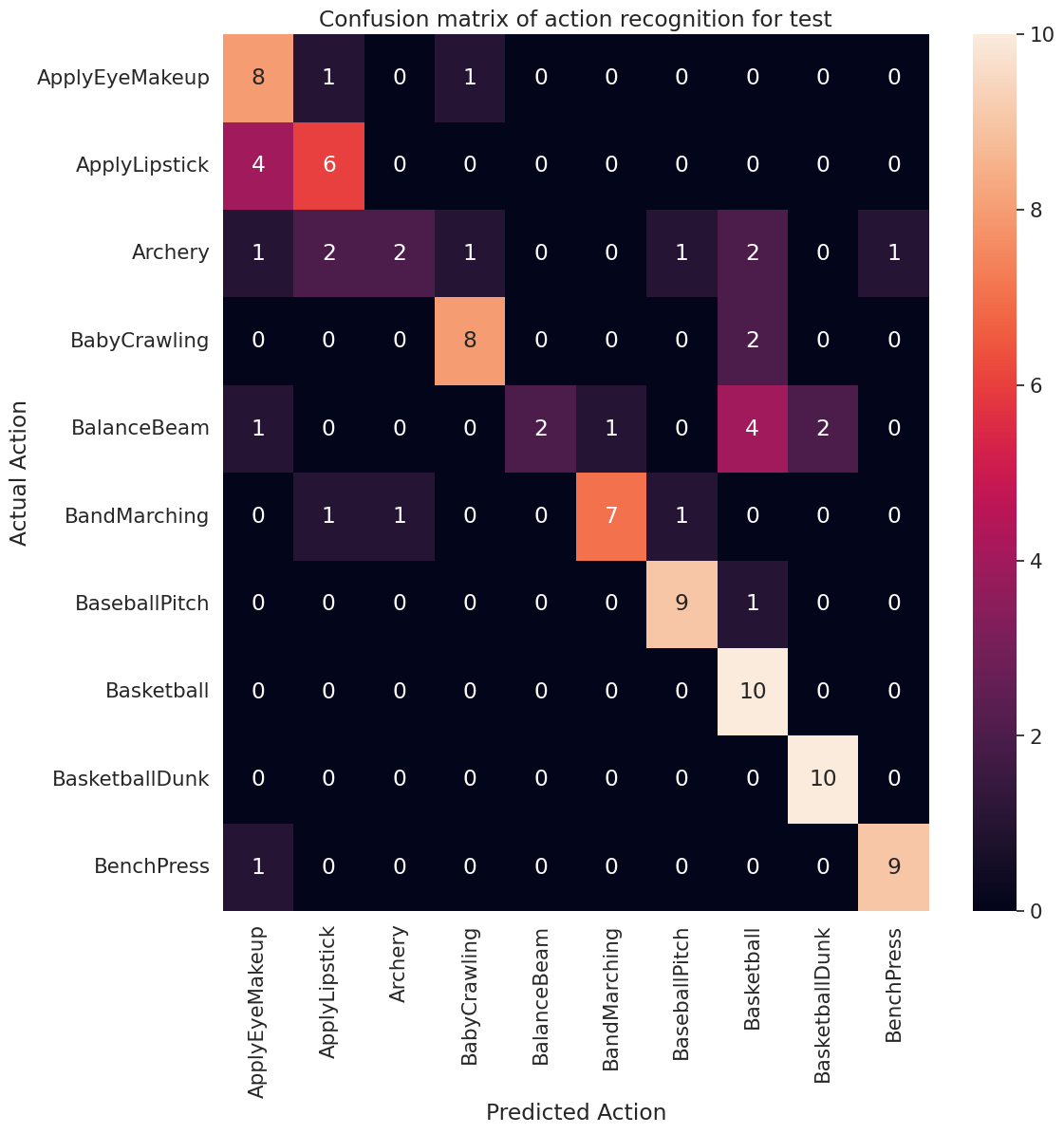
The precision and recall values for each class can also be calculated using a confusion matrix.

def calculate_classification_metrics(y_actual, y_pred, labels):
  """
    Calculate the precision and recall of a classification model using the ground truth and
    predicted values. 

    Args:
      y_actual: Ground truth labels.
      y_pred: Predicted labels.
      labels: List of classification labels.

    Return:
      Precision and recall measures.
  """
  cm = tf.math.confusion_matrix(y_actual, y_pred)
  tp = np.diag(cm) # Diagonal represents true positives
  precision = dict()
  recall = dict()
  for i in range(len(labels)):
    col = cm[:, i]
    fp = np.sum(col) - tp[i] # Sum of column minus true positive is false negative

    row = cm[i, :]
    fn = np.sum(row) - tp[i] # Sum of row minus true positive, is false negative

    precision[labels[i]] = tp[i] / (tp[i] + fp) # Precision 

    recall[labels[i]] = tp[i] / (tp[i] + fn) # Recall

  return precision, recall

precision, recall = calculate_classification_metrics(actual, predicted, labels) # Test dataset

precision

{'ApplyEyeMakeup': 0.5333333333333333,
 'ApplyLipstick': 0.6,
 'Archery': 0.6666666666666666,
 'BabyCrawling': 0.8,
 'BalanceBeam': 1.0,
 'BandMarching': 0.875,
 'BaseballPitch': 0.8181818181818182,
 'Basketball': 0.5263157894736842,
 'BasketballDunk': 0.8333333333333334,
 'BenchPress': 0.9}

recall

{'ApplyEyeMakeup': 0.8,
 'ApplyLipstick': 0.6,
 'Archery': 0.2,
 'BabyCrawling': 0.8,
 'BalanceBeam': 0.2,
 'BandMarching': 0.7,
 'BaseballPitch': 0.9,
 'Basketball': 1.0,
 'BasketballDunk': 1.0,
 'BenchPress': 0.9}

Next steps

To learn more about working with video data in TensorFlow, check out the following tutorials: