
|
|
|
 View source on GitHub
|
|
Overview
This notebook shows how to compress a model using TensorFlow Compression.
In the example below, we compress the weights of an MNIST classifier to a much smaller size than their floating point representation, while retaining classification accuracy. This is done by a two step process, based on the paper Scalable Model Compression by Entropy Penalized Reparameterization:
Training a "compressible" model with an explicit entropy penalty during training, which encourages compressibility of the model parameters. The weight on this penalty, \(\lambda\), enables continuously controlling the trade-off between the compressed model size and its accuracy.
Encoding the compressible model into a compressed model using a coding scheme that is matched with the penalty, meaning that the penalty is a good predictor for model size. This ensures that the method doesn't require multiple iterations of training, compressing, and re-training the model for fine-tuning.
This method is strictly concerned with compressed model size, not with computational complexity. It can be combined with a technique like model pruning to reduce size and complexity.
Example compression results on various models:
| Model (dataset) | Model size | Comp. ratio | Top-1 error comp. (uncomp.) |
|---|---|---|---|
| LeNet300-100 (MNIST) | 8.56 KB | 124x | 1.9% (1.6%) |
| LeNet5-Caffe (MNIST) | 2.84 KB | 606x | 1.0% (0.7%) |
| VGG-16 (CIFAR-10) | 101 KB | 590x | 10.0% (6.6%) |
| ResNet-20-4 (CIFAR-10) | 128 KB | 134x | 8.8% (5.0%) |
| ResNet-18 (ImageNet) | 1.97 MB | 24x | 30.0% (30.0%) |
| ResNet-50 (ImageNet) | 5.49 MB | 19x | 26.0% (25.0%) |
Applications include:
- Deploying/broadcasting models to edge devices on a large scale, saving bandwidth in transit.
- Communicating global model state to clients in federated learning. The model architecture (number of hidden units, etc.) is unchanged from the initial model, and clients can continue learning on the decompressed model.
- Performing inference on extremely memory limited clients. During inference, the weights of each layer can be sequentially decompressed, and discarded right after the activations are computed.
Setup
Install Tensorflow Compression via pip.
# Installs the latest version of TFC compatible with the installed TF version.read MAJOR MINOR <<< "$(pip show tensorflow | perl -p -0777 -e 's/.*Version: (\d+)\.(\d+).*/\1 \2/sg')"pip install "tensorflow-compression<$MAJOR.$(($MINOR+1))"
ERROR: pip's dependency resolver does not currently take into account all the packages that are installed. This behaviour is the source of the following dependency conflicts.
tf-keras 2.17.0 requires tensorflow<2.18,>=2.17, but you have tensorflow 2.14.1 which is incompatible.
Import library dependencies.
import matplotlib.pyplot as plt
import tensorflow as tf
import tensorflow_compression as tfc
import tensorflow_datasets as tfds
2024-08-16 01:51:15.348618: E tensorflow/compiler/xla/stream_executor/cuda/cuda_dnn.cc:9342] Unable to register cuDNN factory: Attempting to register factory for plugin cuDNN when one has already been registered
2024-08-16 01:51:15.348666: E tensorflow/compiler/xla/stream_executor/cuda/cuda_fft.cc:609] Unable to register cuFFT factory: Attempting to register factory for plugin cuFFT when one has already been registered
2024-08-16 01:51:15.348703: E tensorflow/compiler/xla/stream_executor/cuda/cuda_blas.cc:1518] Unable to register cuBLAS factory: Attempting to register factory for plugin cuBLAS when one has already been registered
Define and train a basic MNIST classifier
In order to effectively compress dense and convolutional layers, we need to define custom layer classes. These are analogous to the layers under tf.keras.layers, but we will subclass them later to effectively implement Entropy Penalized Reparameterization (EPR). For this purpose, we also add a copy constructor.
First, we define a standard dense layer:
class CustomDense(tf.keras.layers.Layer):

  def __init__(self, filters, name="dense"):
    super().__init__(name=name)
    self.filters = filters

  @classmethod
  def copy(cls, other, **kwargs):
    """Returns an instantiated and built layer, initialized from `other`."""
    self = cls(filters=other.filters, name=other.name, **kwargs)
    self.build(None, other=other)
    return self

  def build(self, input_shape, other=None):
    """Instantiates weights, optionally initializing them from `other`."""
    if other is None:
      kernel_shape = (input_shape[-1], self.filters)
      kernel = tf.keras.initializers.GlorotUniform()(shape=kernel_shape)
      bias = tf.keras.initializers.Zeros()(shape=(self.filters,))
    else:
      kernel, bias = other.kernel, other.bias
    self.kernel = tf.Variable(
        tf.cast(kernel, self.variable_dtype), name="kernel")
    self.bias = tf.Variable(
        tf.cast(bias, self.variable_dtype), name="bias")
    self.built = True

  def call(self, inputs):
    outputs = tf.linalg.matvec(self.kernel, inputs, transpose_a=True)
    outputs = tf.nn.bias_add(outputs, self.bias)
    return tf.nn.leaky_relu(outputs)
And similarly, a 2D convolutional layer:
class CustomConv2D(tf.keras.layers.Layer):

  def __init__(self, filters, kernel_size,
               strides=1, padding="SAME", name="conv2d"):
    super().__init__(name=name)
    self.filters = filters
    self.kernel_size = kernel_size
    self.strides = strides
    self.padding = padding

  @classmethod
  def copy(cls, other, **kwargs):
    """Returns an instantiated and built layer, initialized from `other`."""
    self = cls(filters=other.filters, kernel_size=other.kernel_size,
               strides=other.strides, padding=other.padding, name=other.name,
               **kwargs)
    self.build(None, other=other)
    return self

  def build(self, input_shape, other=None):
    """Instantiates weights, optionally initializing them from `other`."""
    if other is None:
      kernel_shape = 2 * (self.kernel_size,) + (input_shape[-1], self.filters)
      kernel = tf.keras.initializers.GlorotUniform()(shape=kernel_shape)
      bias = tf.keras.initializers.Zeros()(shape=(self.filters,))
    else:
      kernel, bias = other.kernel, other.bias
    self.kernel = tf.Variable(
        tf.cast(kernel, self.variable_dtype), name="kernel")
    self.bias = tf.Variable(
        tf.cast(bias, self.variable_dtype), name="bias")
    self.built = True

  def call(self, inputs):
    outputs = tf.nn.convolution(
        inputs, self.kernel, strides=self.strides, padding=self.padding)
    outputs = tf.nn.bias_add(outputs, self.bias)
    return tf.nn.leaky_relu(outputs)
Before we continue with model compression, let's check that we can successfully train a regular classifier.
Define the model architecture:
classifier = tf.keras.Sequential([
    CustomConv2D(20, 5, strides=2, name="conv_1"),
    CustomConv2D(50, 5, strides=2, name="conv_2"),
    tf.keras.layers.Flatten(),
    CustomDense(500, name="fc_1"),
    CustomDense(10, name="fc_2"),
], name="classifier")
2024-08-16 01:51:18.645015: W tensorflow/core/common_runtime/gpu/gpu_device.cc:2211] Cannot dlopen some GPU libraries. Please make sure the missing libraries mentioned above are installed properly if you would like to use GPU. Follow the guide at https://www.tensorflow.org/install/gpu for how to download and setup the required libraries for your platform.
Skipping registering GPU devices...
Load the training data:
def normalize_img(image, label):
  """Normalizes images: `uint8` -> `float32`."""
  return tf.cast(image, tf.float32) / 255., label

training_dataset, validation_dataset = tfds.load(
    "mnist",
    split=["train", "test"],
    shuffle_files=True,
    as_supervised=True,
    with_info=False,
)
training_dataset = training_dataset.map(normalize_img)
validation_dataset = validation_dataset.map(normalize_img)
Finally, train the model:
def train_model(model, training_data, validation_data, **kwargs):
  model.compile(
      optimizer=tf.keras.optimizers.Adam(learning_rate=1e-3),
      loss=tf.keras.losses.SparseCategoricalCrossentropy(from_logits=True),
      metrics=[tf.keras.metrics.SparseCategoricalAccuracy()],
      # Uncomment this to ease debugging:
      # run_eagerly=True,
  )
  kwargs.setdefault("epochs", 5)
  kwargs.setdefault("verbose", 1)
  log = model.fit(
      training_data.batch(128).prefetch(8),
      validation_data=validation_data.batch(128).cache(),
      validation_freq=1,
      **kwargs,
  )
  return log.history["val_sparse_categorical_accuracy"][-1]

classifier_accuracy = train_model(
    classifier, training_dataset, validation_dataset)

print(f"Accuracy: {classifier_accuracy:0.4f}")
Epoch 1/5
469/469 [==============================] - 51s 104ms/step - loss: 0.2070 - sparse_categorical_accuracy: 0.9377 - val_loss: 0.0735 - val_sparse_categorical_accuracy: 0.9768
Epoch 2/5
469/469 [==============================] - 48s 103ms/step - loss: 0.0626 - sparse_categorical_accuracy: 0.9809 - val_loss: 0.0611 - val_sparse_categorical_accuracy: 0.9814
Epoch 3/5
469/469 [==============================] - 48s 103ms/step - loss: 0.0428 - sparse_categorical_accuracy: 0.9869 - val_loss: 0.0580 - val_sparse_categorical_accuracy: 0.9815
Epoch 4/5
469/469 [==============================] - 49s 103ms/step - loss: 0.0318 - sparse_categorical_accuracy: 0.9903 - val_loss: 0.0626 - val_sparse_categorical_accuracy: 0.9813
Epoch 5/5
469/469 [==============================] - 49s 104ms/step - loss: 0.0247 - sparse_categorical_accuracy: 0.9923 - val_loss: 0.0546 - val_sparse_categorical_accuracy: 0.9846
Accuracy: 0.9846
Success! The model trained fine, and reached an accuracy of over 98% on the validation set within 5 epochs.
Train a compressible classifier
Entropy Penalized Reparameterization (EPR) has two main ingredients:
Applying a penalty to the model weights during training which corresponds to their entropy under a probabilistic model, which is matched with the encoding scheme of the weights. Below, we define a Keras
Regularizerwhich implements this penalty.Reparameterizing the weights, i.e. bringing them into a latent representation which is more compressible (yields a better trade-off between compressibility and model performance). For convolutional kernels, it has been shown that the Fourier domain is a good representation. For other parameters, the below example simply uses scalar quantization (rounding) with a varying quantization step size.
First, define the penalty.
The example below uses a code/probabilistic model implemented in the tfc.PowerLawEntropyModel class, inspired by the paper Optimizing the Communication-Accuracy Trade-off in Federated Learning with Rate-Distortion Theory. The penalty is defined as:
\[ \log \Bigl(\frac {|x| + \alpha} \alpha\Bigr), \]
where \(x\) is one element of the model parameter or its latent representation, and \(\alpha\) is a small constant for numerical stability around values of 0.
_ = tf.linspace(-5., 5., 501)
plt.plot(_, tfc.PowerLawEntropyModel(0).penalty(_));
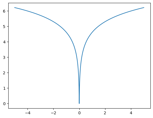
The penalty is effectively a regularization loss (sometimes called "weight loss"). The fact that it is concave with a cusp at zero encourages weight sparsity. The coding scheme applied for compressing the weights, an Elias gamma code, produces codes of length \( 1 + \lfloor \log_2 |x| \rfloor \) bits for the magnitude of the element. That is, it is matched to the penalty, and applying the penalty thus minimizes the expected code length.
class PowerLawRegularizer(tf.keras.regularizers.Regularizer):

  def __init__(self, lmbda):
    super().__init__()
    self.lmbda = lmbda

  def __call__(self, variable):
    em = tfc.PowerLawEntropyModel(coding_rank=variable.shape.rank)
    return self.lmbda * em.penalty(variable)

# Normalizing the weight of the penalty by the number of model parameters is a
# good rule of thumb to produce comparable results across models.
regularizer = PowerLawRegularizer(lmbda=2./classifier.count_params())
Second, define subclasses of CustomDense and CustomConv2D which have the following additional functionality:
- They take an instance of the above regularizer and apply it to the kernels and biases during training.
- They define kernel and bias as a
@property, which perform quantization with straight-through gradients whenever the variables are accessed. This accurately reflects the computation that is carried out later in the compressed model. - They define additional
log_stepvariables, which represent the logarithm of the quantization step size. The coarser the quantization, the smaller the model size, but the lower the accuracy. The quantization step sizes are trainable for each model parameter, so that performing optimization on the penalized loss function will determine what quantization step size is best.
The quantization step is defined as follows:
def quantize(latent, log_step):
  step = tf.exp(log_step)
  return tfc.round_st(latent / step) * step
With that, we can define the dense layer:
class CompressibleDense(CustomDense):

  def __init__(self, regularizer, *args, **kwargs):
    super().__init__(*args, **kwargs)
    self.regularizer = regularizer

  def build(self, input_shape, other=None):
    """Instantiates weights, optionally initializing them from `other`."""
    super().build(input_shape, other=other)
    if other is not None and hasattr(other, "kernel_log_step"):
      kernel_log_step = other.kernel_log_step
      bias_log_step = other.bias_log_step
    else:
      kernel_log_step = bias_log_step = -4.
    self.kernel_log_step = tf.Variable(
        tf.cast(kernel_log_step, self.variable_dtype), name="kernel_log_step")
    self.bias_log_step = tf.Variable(
        tf.cast(bias_log_step, self.variable_dtype), name="bias_log_step")
    self.add_loss(lambda: self.regularizer(
        self.kernel_latent / tf.exp(self.kernel_log_step)))
    self.add_loss(lambda: self.regularizer(
        self.bias_latent / tf.exp(self.bias_log_step)))

  @property
  def kernel(self):
    return quantize(self.kernel_latent, self.kernel_log_step)

  @kernel.setter
  def kernel(self, kernel):
    self.kernel_latent = tf.Variable(kernel, name="kernel_latent")

  @property
  def bias(self):
    return quantize(self.bias_latent, self.bias_log_step)

  @bias.setter
  def bias(self, bias):
    self.bias_latent = tf.Variable(bias, name="bias_latent")
The convolutional layer is analogous. In addition, the convolution kernel is stored as its real-valued discrete Fourier transform (RDFT) whenever the kernel is set, and the transform is inverted whenever the kernel is used. Since the different frequency components of the kernel tend to be more or less compressible, each of them gets its own quantization step size assigned.
Define the Fourier transform and its inverse as follows:
def to_rdft(kernel, kernel_size):
  # The kernel has shape (H, W, I, O) -> transpose to take DFT over last two
  # dimensions.
  kernel = tf.transpose(kernel, (2, 3, 0, 1))
  # The RDFT has type complex64 and shape (I, O, FH, FW).
  kernel_rdft = tf.signal.rfft2d(kernel)
  # Map real and imaginary parts into regular floats. The result is float32
  # and has shape (I, O, FH, FW, 2).
  kernel_rdft = tf.stack(
      [tf.math.real(kernel_rdft), tf.math.imag(kernel_rdft)], axis=-1)
  # Divide by kernel size to make the DFT orthonormal (length-preserving).
  return kernel_rdft / kernel_size

def from_rdft(kernel_rdft, kernel_size):
  # Undoes the transformations in to_rdft.
  kernel_rdft *= kernel_size
  kernel_rdft = tf.dtypes.complex(*tf.unstack(kernel_rdft, axis=-1))
  kernel = tf.signal.irfft2d(kernel_rdft, fft_length=2 * (kernel_size,))
  return tf.transpose(kernel, (2, 3, 0, 1))
With that, define the convolutional layer as:
class CompressibleConv2D(CustomConv2D):

  def __init__(self, regularizer, *args, **kwargs):
    super().__init__(*args, **kwargs)
    self.regularizer = regularizer

  def build(self, input_shape, other=None):
    """Instantiates weights, optionally initializing them from `other`."""
    super().build(input_shape, other=other)
    if other is not None and hasattr(other, "kernel_log_step"):
      kernel_log_step = other.kernel_log_step
      bias_log_step = other.bias_log_step
    else:
      kernel_log_step = tf.fill(self.kernel_latent.shape[2:], -4.)
      bias_log_step = -4.
    self.kernel_log_step = tf.Variable(
        tf.cast(kernel_log_step, self.variable_dtype), name="kernel_log_step")
    self.bias_log_step = tf.Variable(
        tf.cast(bias_log_step, self.variable_dtype), name="bias_log_step")
    self.add_loss(lambda: self.regularizer(
        self.kernel_latent / tf.exp(self.kernel_log_step)))
    self.add_loss(lambda: self.regularizer(
        self.bias_latent / tf.exp(self.bias_log_step)))

  @property
  def kernel(self):
    kernel_rdft = quantize(self.kernel_latent, self.kernel_log_step)
    return from_rdft(kernel_rdft, self.kernel_size)

  @kernel.setter
  def kernel(self, kernel):
    kernel_rdft = to_rdft(kernel, self.kernel_size)
    self.kernel_latent = tf.Variable(kernel_rdft, name="kernel_latent")

  @property
  def bias(self):
    return quantize(self.bias_latent, self.bias_log_step)

  @bias.setter
  def bias(self, bias):
    self.bias_latent = tf.Variable(bias, name="bias_latent")
Define a classifier model with the same architecture as above, but using these modified layers:
def make_mnist_classifier(regularizer):
  return tf.keras.Sequential([
      CompressibleConv2D(regularizer, 20, 5, strides=2, name="conv_1"),
      CompressibleConv2D(regularizer, 50, 5, strides=2, name="conv_2"),
      tf.keras.layers.Flatten(),
      CompressibleDense(regularizer, 500, name="fc_1"),
      CompressibleDense(regularizer, 10, name="fc_2"),
  ], name="classifier")

compressible_classifier = make_mnist_classifier(regularizer)
And train the model:
penalized_accuracy = train_model(
    compressible_classifier, training_dataset, validation_dataset)

print(f"Accuracy: {penalized_accuracy:0.4f}")
Epoch 1/5
469/469 [==============================] - 54s 111ms/step - loss: 3.8076 - sparse_categorical_accuracy: 0.9307 - val_loss: 2.1789 - val_sparse_categorical_accuracy: 0.9741
Epoch 2/5
469/469 [==============================] - 52s 111ms/step - loss: 1.6671 - sparse_categorical_accuracy: 0.9768 - val_loss: 1.2815 - val_sparse_categorical_accuracy: 0.9822
Epoch 3/5
469/469 [==============================] - 52s 111ms/step - loss: 1.0644 - sparse_categorical_accuracy: 0.9835 - val_loss: 0.9371 - val_sparse_categorical_accuracy: 0.9846
Epoch 4/5
469/469 [==============================] - 52s 112ms/step - loss: 0.7908 - sparse_categorical_accuracy: 0.9865 - val_loss: 0.7463 - val_sparse_categorical_accuracy: 0.9853
Epoch 5/5
469/469 [==============================] - 52s 111ms/step - loss: 0.6484 - sparse_categorical_accuracy: 0.9879 - val_loss: 0.6469 - val_sparse_categorical_accuracy: 0.9857
Accuracy: 0.9857
The compressible model has reached a similar accuracy as the plain classifier.
However, the model is not actually compressed yet. To do this, we define another set of subclasses which store the kernels and biases in their compressed form – as a sequence of bits.
Compress the classifier
The subclasses of CustomDense and CustomConv2D defined below convert the weights of a compressible dense layer into binary strings. In addition, they store the logarithm of the quantization step size at half precision to save space. Whenever the kernel or bias is accessed through the @property, they are decompressed from their string representation and dequantized.
First, define functions to compress and decompress a model parameter:
def compress_latent(latent, log_step, name):
  em = tfc.PowerLawEntropyModel(latent.shape.rank)
  compressed = em.compress(latent / tf.exp(log_step))
  compressed = tf.Variable(compressed, name=f"{name}_compressed")
  log_step = tf.cast(log_step, tf.float16)
  log_step = tf.Variable(log_step, name=f"{name}_log_step")
  return compressed, log_step

def decompress_latent(compressed, shape, log_step):
  latent = tfc.PowerLawEntropyModel(len(shape)).decompress(compressed, shape)
  step = tf.exp(tf.cast(log_step, latent.dtype))
  return latent * step
With these, we can define CompressedDense:
class CompressedDense(CustomDense):

  def build(self, input_shape, other=None):
    assert isinstance(other, CompressibleDense)
    self.input_channels = other.kernel.shape[0]
    self.kernel_compressed, self.kernel_log_step = compress_latent(
        other.kernel_latent, other.kernel_log_step, "kernel")
    self.bias_compressed, self.bias_log_step = compress_latent(
        other.bias_latent, other.bias_log_step, "bias")
    self.built = True

  @property
  def kernel(self):
    kernel_shape = (self.input_channels, self.filters)
    return decompress_latent(
        self.kernel_compressed, kernel_shape, self.kernel_log_step)

  @property
  def bias(self):
    bias_shape = (self.filters,)
    return decompress_latent(
        self.bias_compressed, bias_shape, self.bias_log_step)
The convolutional layer class is analogous to the above.
class CompressedConv2D(CustomConv2D):

  def build(self, input_shape, other=None):
    assert isinstance(other, CompressibleConv2D)
    self.input_channels = other.kernel.shape[2]
    self.kernel_compressed, self.kernel_log_step = compress_latent(
        other.kernel_latent, other.kernel_log_step, "kernel")
    self.bias_compressed, self.bias_log_step = compress_latent(
        other.bias_latent, other.bias_log_step, "bias")
    self.built = True

  @property
  def kernel(self):
    rdft_shape = (self.input_channels, self.filters,
                  self.kernel_size, self.kernel_size // 2 + 1, 2)
    kernel_rdft = decompress_latent(
        self.kernel_compressed, rdft_shape, self.kernel_log_step)
    return from_rdft(kernel_rdft, self.kernel_size)

  @property
  def bias(self):
    bias_shape = (self.filters,)
    return decompress_latent(
        self.bias_compressed, bias_shape, self.bias_log_step)
To turn the compressible model into a compressed one, we can conveniently use the clone_model function. compress_layer converts any compressible layer into a compressed one, and simply passes through any other types of layers (such as Flatten, etc.).
def compress_layer(layer):
  if isinstance(layer, CompressibleDense):
    return CompressedDense.copy(layer)
  if isinstance(layer, CompressibleConv2D):
    return CompressedConv2D.copy(layer)
  return type(layer).from_config(layer.get_config())

compressed_classifier = tf.keras.models.clone_model(
    compressible_classifier, clone_function=compress_layer)
Now, let's validate that the compressed model still performs as expected:
compressed_classifier.compile(metrics=[tf.keras.metrics.SparseCategoricalAccuracy()])
_, compressed_accuracy = compressed_classifier.evaluate(validation_dataset.batch(128))

print(f"Accuracy of the compressible classifier: {penalized_accuracy:0.4f}")
print(f"Accuracy of the compressed classifier: {compressed_accuracy:0.4f}")
79/79 [==============================] - 1s 10ms/step - loss: 0.0000e+00 - sparse_categorical_accuracy: 0.9857
Accuracy of the compressible classifier: 0.9857
Accuracy of the compressed classifier: 0.9857
The classification accuracy of the compressed model is identical to the one achieved during training!
In addition, the size of the compressed model weights is much smaller than the original model size:
def get_weight_size_in_bytes(weight):
  if weight.dtype == tf.string:
    return tf.reduce_sum(tf.strings.length(weight, unit="BYTE"))
  else:
    return tf.size(weight) * weight.dtype.size

original_size = sum(map(get_weight_size_in_bytes, classifier.weights))
compressed_size = sum(map(get_weight_size_in_bytes, compressed_classifier.weights))

print(f"Size of original model weights: {original_size} bytes")
print(f"Size of compressed model weights: {compressed_size} bytes")
print(f"Compression ratio: {(original_size/compressed_size):0.0f}x")
Size of original model weights: 5024320 bytes
Size of compressed model weights: 19047 bytes
Compression ratio: 264x
Storing the models on disk requires some overhead for storing the model architecture, function graphs, etc.
Lossless compression methods such as ZIP are good at compressing this type of data, but not the weights themselves. That is why there is still a significant benefit of EPR when counting model size inclusive of that overhead, after also applying ZIP compression:
import os
import shutil

def get_disk_size(model, path):
  model.save(path)
  zip_path = shutil.make_archive(path, "zip", path)
  return os.path.getsize(zip_path)

original_zip_size = get_disk_size(classifier, "/tmp/classifier")
compressed_zip_size = get_disk_size(
    compressed_classifier, "/tmp/compressed_classifier")

print(f"Original on-disk size (ZIP compressed): {original_zip_size} bytes")
print(f"Compressed on-disk size (ZIP compressed): {compressed_zip_size} bytes")
print(f"Compression ratio: {(original_zip_size/compressed_zip_size):0.0f}x")
INFO:tensorflow:Assets written to: /tmp/classifier/assets
INFO:tensorflow:Assets written to: /tmp/classifier/assets
INFO:tensorflow:Assets written to: /tmp/compressed_classifier/assets
INFO:tensorflow:Assets written to: /tmp/compressed_classifier/assets
Original on-disk size (ZIP compressed): 13906833 bytes
Compressed on-disk size (ZIP compressed): 61183 bytes
Compression ratio: 227x
Regularization effect and size–accuracy trade-off
Above, the \(\lambda\) hyperparameter was set to 2 (normalized by the number of parameters in the model). As we increase \(\lambda\), the model weights are more and more heavily penalized for compressibility.
For low values, the penalty can act like a weight regularizer. It actually has a beneficial effect on the generalization performance of the classifier, and can lead to a slightly higher accuracy on the validation dataset:
print(f"Accuracy of the vanilla classifier: {classifier_accuracy:0.4f}")
print(f"Accuracy of the penalized classifier: {penalized_accuracy:0.4f}")
Accuracy of the vanilla classifier: 0.9846
Accuracy of the penalized classifier: 0.9857
For higher values, we see a smaller and smaller model size, but also a gradually diminishing accuracy. To see this, let's train a few models and plot their size vs. accuracy:
def compress_and_evaluate_model(lmbda):
  print(f"lambda={lmbda:0.0f}: training...", flush=True)
  regularizer = PowerLawRegularizer(lmbda=lmbda/classifier.count_params())
  compressible_classifier = make_mnist_classifier(regularizer)
  train_model(
      compressible_classifier, training_dataset, validation_dataset, verbose=0)
  print("compressing...", flush=True)
  compressed_classifier = tf.keras.models.clone_model(
      compressible_classifier, clone_function=compress_layer)
  compressed_size = sum(map(
      get_weight_size_in_bytes, compressed_classifier.weights))
  compressed_zip_size = float(get_disk_size(
      compressed_classifier, "/tmp/compressed_classifier"))
  print("evaluating...", flush=True)
  compressed_classifier = tf.keras.models.load_model(
      "/tmp/compressed_classifier")
  compressed_classifier.compile(
      metrics=[tf.keras.metrics.SparseCategoricalAccuracy()])
  _, compressed_accuracy = compressed_classifier.evaluate(
      validation_dataset.batch(128), verbose=0)
  print()
  return compressed_size, compressed_zip_size, compressed_accuracy

lambdas = (2., 5., 10., 20., 50.)
metrics = [compress_and_evaluate_model(l) for l in lambdas]
metrics = tf.convert_to_tensor(metrics, tf.float32)
lambda=2: training...
compressing...
WARNING:tensorflow:Compiled the loaded model, but the compiled metrics have yet to be built. `model.compile_metrics` will be empty until you train or evaluate the model.
WARNING:tensorflow:Compiled the loaded model, but the compiled metrics have yet to be built. `model.compile_metrics` will be empty until you train or evaluate the model.
INFO:tensorflow:Assets written to: /tmp/compressed_classifier/assets
INFO:tensorflow:Assets written to: /tmp/compressed_classifier/assets
evaluating...
WARNING:tensorflow:No training configuration found in save file, so the model was *not* compiled. Compile it manually.
WARNING:tensorflow:No training configuration found in save file, so the model was *not* compiled. Compile it manually.
lambda=5: training...
compressing...
WARNING:tensorflow:Compiled the loaded model, but the compiled metrics have yet to be built. `model.compile_metrics` will be empty until you train or evaluate the model.
WARNING:tensorflow:Compiled the loaded model, but the compiled metrics have yet to be built. `model.compile_metrics` will be empty until you train or evaluate the model.
INFO:tensorflow:Assets written to: /tmp/compressed_classifier/assets
INFO:tensorflow:Assets written to: /tmp/compressed_classifier/assets
evaluating...
WARNING:tensorflow:No training configuration found in save file, so the model was *not* compiled. Compile it manually.
WARNING:tensorflow:No training configuration found in save file, so the model was *not* compiled. Compile it manually.
lambda=10: training...
compressing...
WARNING:tensorflow:Compiled the loaded model, but the compiled metrics have yet to be built. `model.compile_metrics` will be empty until you train or evaluate the model.
WARNING:tensorflow:Compiled the loaded model, but the compiled metrics have yet to be built. `model.compile_metrics` will be empty until you train or evaluate the model.
INFO:tensorflow:Assets written to: /tmp/compressed_classifier/assets
INFO:tensorflow:Assets written to: /tmp/compressed_classifier/assets
evaluating...
WARNING:tensorflow:No training configuration found in save file, so the model was *not* compiled. Compile it manually.
WARNING:tensorflow:No training configuration found in save file, so the model was *not* compiled. Compile it manually.
lambda=20: training...
compressing...
WARNING:tensorflow:Compiled the loaded model, but the compiled metrics have yet to be built. `model.compile_metrics` will be empty until you train or evaluate the model.
WARNING:tensorflow:Compiled the loaded model, but the compiled metrics have yet to be built. `model.compile_metrics` will be empty until you train or evaluate the model.
INFO:tensorflow:Assets written to: /tmp/compressed_classifier/assets
INFO:tensorflow:Assets written to: /tmp/compressed_classifier/assets
evaluating...
WARNING:tensorflow:No training configuration found in save file, so the model was *not* compiled. Compile it manually.
WARNING:tensorflow:No training configuration found in save file, so the model was *not* compiled. Compile it manually.
lambda=50: training...
compressing...
WARNING:tensorflow:Compiled the loaded model, but the compiled metrics have yet to be built. `model.compile_metrics` will be empty until you train or evaluate the model.
WARNING:tensorflow:Compiled the loaded model, but the compiled metrics have yet to be built. `model.compile_metrics` will be empty until you train or evaluate the model.
INFO:tensorflow:Assets written to: /tmp/compressed_classifier/assets
INFO:tensorflow:Assets written to: /tmp/compressed_classifier/assets
evaluating...
WARNING:tensorflow:No training configuration found in save file, so the model was *not* compiled. Compile it manually.
WARNING:tensorflow:No training configuration found in save file, so the model was *not* compiled. Compile it manually.
def plot_broken_xaxis(ax, compressed_sizes, original_size, original_accuracy):
  xticks = list(range(
      int(tf.math.floor(min(compressed_sizes) / 5) * 5),
      int(tf.math.ceil(max(compressed_sizes) / 5) * 5) + 1,
      5))
  xticks.append(xticks[-1] + 10)
  ax.set_xlim(xticks[0], xticks[-1] + 2)
  ax.set_xticks(xticks[1:])
  ax.set_xticklabels(xticks[1:-1] + [f"{original_size:0.2f}"])
  ax.plot(xticks[-1], original_accuracy, "o", label="float32")

sizes, zip_sizes, accuracies = tf.transpose(metrics)
sizes /= 1024
zip_sizes /= 1024

fig, (axl, axr) = plt.subplots(1, 2, sharey=True, figsize=(10, 4))
axl.plot(sizes, accuracies, "o-", label="EPR compressed")
axr.plot(zip_sizes, accuracies, "o-", label="EPR compressed")
plot_broken_xaxis(axl, sizes, original_size/1024, classifier_accuracy)
plot_broken_xaxis(axr, zip_sizes, original_zip_size/1024, classifier_accuracy)

axl.set_xlabel("size of model weights [kbytes]")
axr.set_xlabel("ZIP compressed on-disk model size [kbytes]")
axl.set_ylabel("accuracy")
axl.legend(loc="lower right")
axr.legend(loc="lower right")
axl.grid()
axr.grid()
for i in range(len(lambdas)):
  axl.annotate(f"$\lambda = {lambdas[i]:0.0f}$", (sizes[i], accuracies[i]),
               xytext=(10, -5), xycoords="data", textcoords="offset points")
  axr.annotate(f"$\lambda = {lambdas[i]:0.0f}$", (zip_sizes[i], accuracies[i]),
               xytext=(10, -5), xycoords="data", textcoords="offset points")
plt.tight_layout()
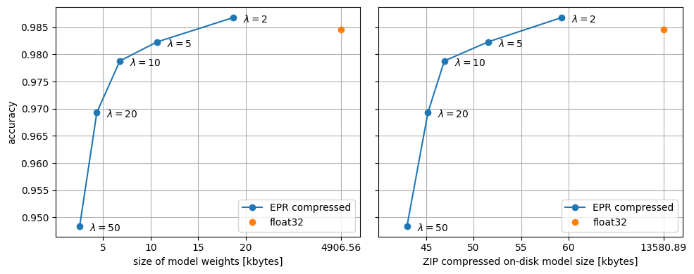
The plot should ideally show an elbow-shaped size–accuracy trade-off, but it is normal for accuracy metrics to be somewhat noisy. Depending on initialization, the curve can exhibit some kinks.
Due to the regularization effect, the EPR compressed model is more accurate on the test set than the original model for small values of \(\lambda\). The EPR compressed model is also many times smaller, even if we compare the sizes after additional ZIP compression.
Decompress the classifier
CompressedDense and CompressedConv2D decompress their weights on every forward pass. This makes them ideal for memory-limited devices, but the decompression can be computationally expensive, especially for small batch sizes.
To decompress the model once, and use it for further training or inference, we can convert it back into a model using regular or compressible layers. This can be useful in model deployment or federated learning scenarios.
First, converting back into a plain model, we can do inference, and/or continue regular training without a compression penalty:
def decompress_layer(layer):
  if isinstance(layer, CompressedDense):
    return CustomDense.copy(layer)
  if isinstance(layer, CompressedConv2D):
    return CustomConv2D.copy(layer)
  return type(layer).from_config(layer.get_config())

decompressed_classifier = tf.keras.models.clone_model(
    compressed_classifier, clone_function=decompress_layer)
decompressed_accuracy = train_model(
    decompressed_classifier, training_dataset, validation_dataset, epochs=1)

print(f"Accuracy of the compressed classifier: {compressed_accuracy:0.4f}")
print(f"Accuracy of the decompressed classifier after one more epoch of training: {decompressed_accuracy:0.4f}")
469/469 [==============================] - 50s 105ms/step - loss: 0.0788 - sparse_categorical_accuracy: 0.9760 - val_loss: 0.0601 - val_sparse_categorical_accuracy: 0.9797
Accuracy of the compressed classifier: 0.9857
Accuracy of the decompressed classifier after one more epoch of training: 0.9797
Note that the validation accuracy drops after training for an additional epoch, since the training is done without regularization.
Alternatively, we can convert the model back into a "compressible" one, for inference and/or further training with a compression penalty:
def decompress_layer_with_penalty(layer):
  if isinstance(layer, CompressedDense):
    return CompressibleDense.copy(layer, regularizer=regularizer)
  if isinstance(layer, CompressedConv2D):
    return CompressibleConv2D.copy(layer, regularizer=regularizer)
  return type(layer).from_config(layer.get_config())

decompressed_classifier = tf.keras.models.clone_model(
    compressed_classifier, clone_function=decompress_layer_with_penalty)
decompressed_accuracy = train_model(
    decompressed_classifier, training_dataset, validation_dataset, epochs=1)

print(f"Accuracy of the compressed classifier: {compressed_accuracy:0.4f}")
print(f"Accuracy of the decompressed classifier after one more epoch of training: {decompressed_accuracy:0.4f}")
469/469 [==============================] - 55s 112ms/step - loss: 0.7432 - sparse_categorical_accuracy: 0.9900 - val_loss: 0.7575 - val_sparse_categorical_accuracy: 0.9872
Accuracy of the compressed classifier: 0.9857
Accuracy of the decompressed classifier after one more epoch of training: 0.9872
Here, the accuracy improves after training for an additional epoch.