
| | |  ดูบน GitHub ดูบน GitHub | | |
บทช่วยสอนนี้ใช้การเรียนรู้เชิงลึกในการเขียนภาพหนึ่งภาพในสไตล์ของอีกภาพหนึ่ง (เคยคิดไหมว่าคุณจะวาดภาพเหมือน Picasso หรือ Van Gogh ได้) สิ่งนี้เรียกว่า การถ่ายโอนสไตล์ประสาท และเทคนิคนี้ได้รับการอธิบายไว้ใน A Neural Algorithm of Artistic Style (Gatys et al.)
สำหรับการประยุกต์ใช้การถ่ายโอนสไตล์อย่างง่าย โปรดดูบทช่วย สอน นี้เพื่อเรียนรู้เพิ่มเติมเกี่ยวกับวิธีใช้ โมเดล Arbitrary Image Stylization ที่ผ่านการฝึกอบรมล่วงหน้าจาก TensorFlow Hub หรือวิธีใช้โมเดลการถ่ายโอนสไตล์กับ TensorFlow Lite
การถ่ายโอนสไตล์ประสาทเป็นเทคนิคการเพิ่มประสิทธิภาพที่ใช้ในการถ่ายภาพสองภาพ—ภาพ เนื้อหา และภาพ อ้างอิงสไตล์ (เช่น งานศิลปะโดยจิตรกรที่มีชื่อเสียง)—และผสมผสานเข้าด้วยกันเพื่อให้ภาพที่ส่งออกดูเหมือนภาพเนื้อหา แต่ "ทาสี" ในรูปแบบของภาพอ้างอิงสไตล์
การดำเนินการนี้ทำได้โดยการเพิ่มประสิทธิภาพรูปภาพที่ส่งออกให้ตรงกับสถิติเนื้อหาของรูปภาพเนื้อหาและสถิติรูปแบบของรูปภาพอ้างอิงสไตล์ สถิติเหล่านี้ดึงมาจากภาพโดยใช้เครือข่ายแบบหมุนวน
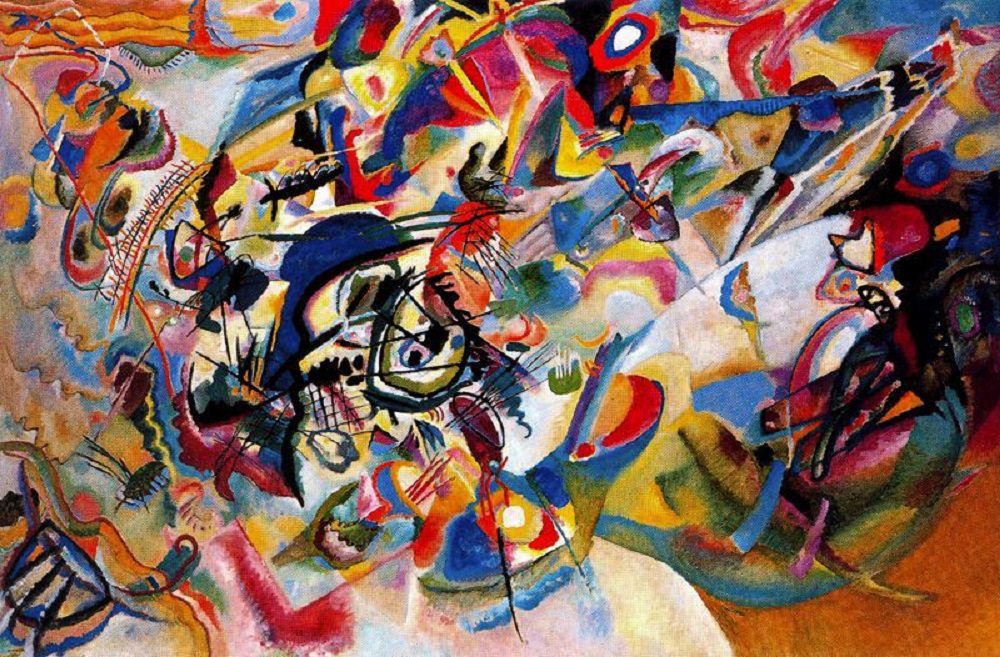
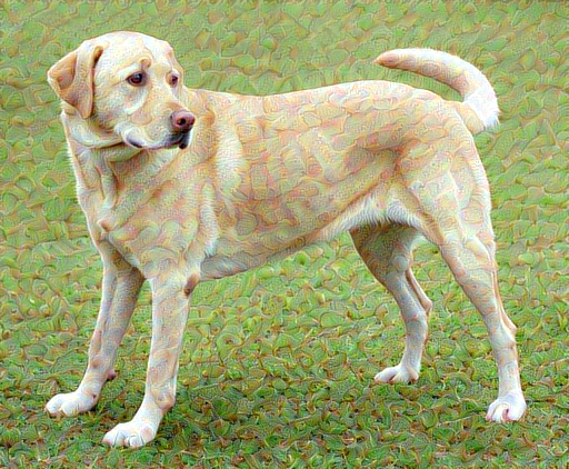
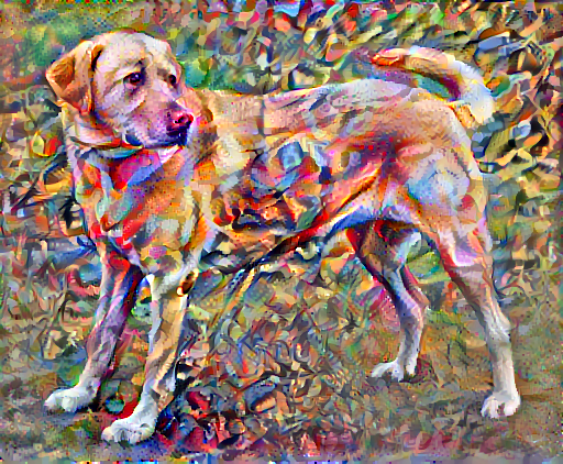
ตัวอย่างเช่น ลองถ่ายรูปสุนัขตัวนี้และ Wassily Kandinsky's Composition 7:

Yellow Labrador Look จาก Wikimedia Commons โดย Elf ใบอนุญาต CC BY-SA 3.0
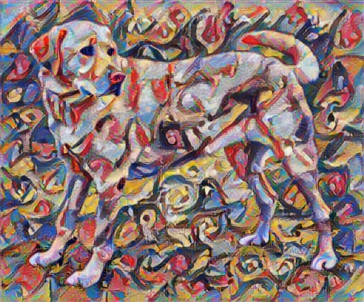
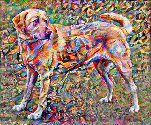
ตอนนี้จะเป็นอย่างไรถ้า Kandinsky ตัดสินใจวาดภาพสุนัขตัวนี้ด้วยสไตล์นี้โดยเฉพาะ? แบบนี้บ้าง?
ติดตั้ง
นำเข้าและกำหนดค่าโมดูล
import os
import tensorflow as tf
# Load compressed models from tensorflow_hub
os.environ['TFHUB_MODEL_LOAD_FORMAT'] = 'COMPRESSED'
import IPython.display as display

import matplotlib.pyplot as plt
import matplotlib as mpl
mpl.rcParams['figure.figsize'] = (12, 12)
mpl.rcParams['axes.grid'] = False

import numpy as np
import PIL.Image
import time
import functools
def tensor_to_image(tensor):
  tensor = tensor*255
  tensor = np.array(tensor, dtype=np.uint8)
  if np.ndim(tensor)>3:
    assert tensor.shape[0] == 1
    tensor = tensor[0]
  return PIL.Image.fromarray(tensor)
ดาวน์โหลดรูปภาพและเลือกรูปภาพสไตล์และรูปภาพเนื้อหา:
content_path = tf.keras.utils.get_file('YellowLabradorLooking_new.jpg', 'https://storage.googleapis.com/download.tensorflow.org/example_images/YellowLabradorLooking_new.jpg')
style_path = tf.keras.utils.get_file('kandinsky5.jpg','https://storage.googleapis.com/download.tensorflow.org/example_images/Vassily_Kandinsky%2C_1913_-_Composition_7.jpg')
Downloading data from https://storage.googleapis.com/download.tensorflow.org/example_images/Vassily_Kandinsky%2C_1913_-_Composition_7.jpg
196608/195196 [==============================] - 0s 0us/step
204800/195196 [===============================] - 0s 0us/step
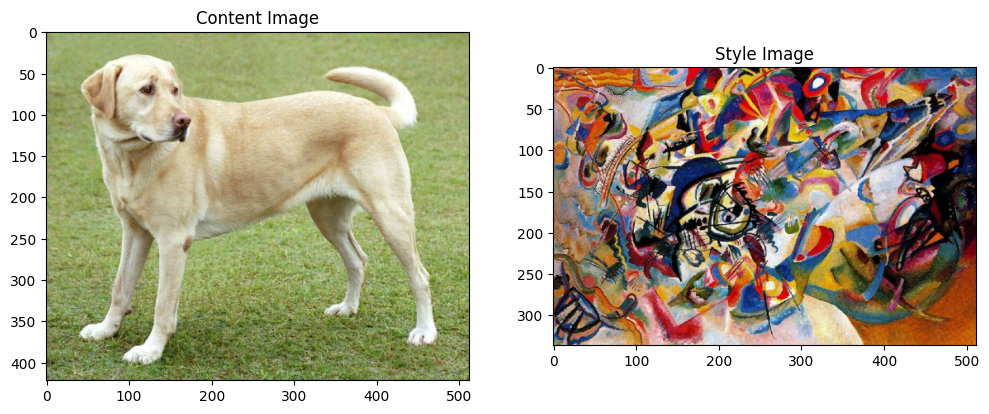
เห็นภาพอินพุต
กำหนดฟังก์ชันเพื่อโหลดรูปภาพและจำกัดขนาดสูงสุดไว้ที่ 512 พิกเซล
def load_img(path_to_img):
  max_dim = 512
  img = tf.io.read_file(path_to_img)
  img = tf.image.decode_image(img, channels=3)
  img = tf.image.convert_image_dtype(img, tf.float32)

  shape = tf.cast(tf.shape(img)[:-1], tf.float32)
  long_dim = max(shape)
  scale = max_dim / long_dim

  new_shape = tf.cast(shape * scale, tf.int32)

  img = tf.image.resize(img, new_shape)
  img = img[tf.newaxis, :]
  return img
สร้างฟังก์ชันง่ายๆ เพื่อแสดงรูปภาพ:
def imshow(image, title=None):
  if len(image.shape) > 3:
    image = tf.squeeze(image, axis=0)

  plt.imshow(image)
  if title:
    plt.title(title)
content_image = load_img(content_path)
style_image = load_img(style_path)

plt.subplot(1, 2, 1)
imshow(content_image, 'Content Image')

plt.subplot(1, 2, 2)
imshow(style_image, 'Style Image')
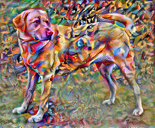
โอนสไตล์อย่างรวดเร็วโดยใช้ TF-Hub
บทช่วยสอนนี้สาธิตอัลกอริธึมการถ่ายโอนสไตล์ดั้งเดิม ซึ่งปรับเนื้อหารูปภาพให้เหมาะสมกับสไตล์เฉพาะ ก่อนจะลงรายละเอียด เรามาดูกันว่า โมเดล TensorFlow Hub ทำได้อย่างไร:
import tensorflow_hub as hub
hub_model = hub.load('https://tfhub.dev/google/magenta/arbitrary-image-stylization-v1-256/2')
stylized_image = hub_model(tf.constant(content_image), tf.constant(style_image))[0]
tensor_to_image(stylized_image)
กำหนดการแสดงเนื้อหาและรูปแบบ
ใช้เลเยอร์ตรงกลางของโมเดลเพื่อรับ เนื้อหา และการนำเสนอ สไตล์ ของรูปภาพ เริ่มจากชั้นอินพุตของเครือข่าย การเปิดใช้งานสองสามชั้นแรกแสดงถึงคุณลักษณะระดับต่ำ เช่น ขอบและพื้นผิว เมื่อคุณก้าวผ่านเครือข่าย เลเยอร์สองสามชั้นสุดท้ายจะแสดงคุณลักษณะระดับสูง เช่น ชิ้นส่วนของวัตถุ เช่น ล้อ หรือ ตา ในกรณีนี้ คุณกำลังใช้สถาปัตยกรรมเครือข่าย VGG19 ซึ่งเป็นเครือข่ายการจัดประเภทรูปภาพที่ได้รับการฝึกอบรมล่วงหน้า เลเยอร์กลางเหล่านี้จำเป็นสำหรับกำหนดการแสดงเนื้อหาและสไตล์จากรูปภาพ สำหรับภาพที่ป้อนเข้า ให้พยายามจับคู่รูปแบบที่สอดคล้องกันและการนำเสนอเป้าหมายของเนื้อหาที่เลเยอร์ระดับกลางเหล่านี้
โหลด VGG19 และทดสอบรันบนอิมเมจของเราเพื่อให้แน่ใจว่าใช้อย่างถูกต้อง:
x = tf.keras.applications.vgg19.preprocess_input(content_image*255)
x = tf.image.resize(x, (224, 224))
vgg = tf.keras.applications.VGG19(include_top=True, weights='imagenet')
prediction_probabilities = vgg(x)
prediction_probabilities.shape
Downloading data from https://storage.googleapis.com/tensorflow/keras-applications/vgg19/vgg19_weights_tf_dim_ordering_tf_kernels.h5
574717952/574710816 [==============================] - 17s 0us/step
574726144/574710816 [==============================] - 17s 0us/step
TensorShape([1, 1000])
predicted_top_5 = tf.keras.applications.vgg19.decode_predictions(prediction_probabilities.numpy())[0]
[(class_name, prob) for (number, class_name, prob) in predicted_top_5]
[('Labrador_retriever', 0.493171),
 ('golden_retriever', 0.2366529),
 ('kuvasz', 0.036357544),
 ('Chesapeake_Bay_retriever', 0.024182785),
 ('Greater_Swiss_Mountain_dog', 0.0186461)]
ตอนนี้โหลด VGG19 โดยไม่มีส่วนหัวของการจัดหมวดหมู่ และแสดงรายการชื่อเลเยอร์
vgg = tf.keras.applications.VGG19(include_top=False, weights='imagenet')

print()
for layer in vgg.layers:
  print(layer.name)
Downloading data from https://storage.googleapis.com/tensorflow/keras-applications/vgg19/vgg19_weights_tf_dim_ordering_tf_kernels_notop.h5
80142336/80134624 [==============================] - 2s 0us/step
80150528/80134624 [==============================] - 2s 0us/step

input_2
block1_conv1
block1_conv2
block1_pool
block2_conv1
block2_conv2
block2_pool
block3_conv1
block3_conv2
block3_conv3
block3_conv4
block3_pool
block4_conv1
block4_conv2
block4_conv3
block4_conv4
block4_pool
block5_conv1
block5_conv2
block5_conv3
block5_conv4
block5_pool
เลือกเลเยอร์กลางจากเครือข่ายเพื่อแสดงสไตล์และเนื้อหาของรูปภาพ:
content_layers = ['block5_conv2']

style_layers = ['block1_conv1',
                'block2_conv1',
                'block3_conv1',
                'block4_conv1',
                'block5_conv1']

num_content_layers = len(content_layers)
num_style_layers = len(style_layers)
เลเยอร์ระดับกลางสำหรับสไตล์และเนื้อหา
เหตุใดเอาต์พุตระดับกลางเหล่านี้ภายในเครือข่ายการจัดประเภทรูปภาพที่ได้รับการฝึกอบรมล่วงหน้าของเราจึงทำให้เราสามารถกำหนดรูปแบบและการแสดงเนื้อหาได้
ในระดับสูง เพื่อให้เครือข่ายทำการจำแนกภาพได้ (ซึ่งเครือข่ายนี้ได้รับการฝึกฝนให้ทำ) เครือข่ายจะต้องเข้าใจภาพ สิ่งนี้ต้องใช้ภาพดิบเป็นพิกเซลอินพุตและสร้างการแสดงภายในที่แปลงพิกเซลภาพดิบเป็นความเข้าใจที่ซับซ้อนของคุณสมบัติที่มีอยู่ในภาพ
นี่เป็นเหตุผลว่าทำไมโครงข่ายประสาทเทียมจึงสามารถสรุปได้ดี: พวกเขาสามารถจับค่าคงที่และกำหนดคุณลักษณะภายในคลาส (เช่น แมวกับสุนัข) ที่ไม่เชื่อเรื่องเสียงพื้นหลังและความรำคาญอื่นๆ ดังนั้น ณ จุดใดจุดหนึ่งระหว่างที่อิมเมจดิบถูกป้อนลงในโมเดลและป้ายกำกับการจัดประเภทเอาต์พุต โมเดลทำหน้าที่เป็นตัวแยกคุณลักษณะที่ซับซ้อน เมื่อเข้าถึงเลเยอร์ตรงกลางของโมเดล คุณจะสามารถอธิบายเนื้อหาและรูปแบบของรูปภาพที่ป้อนได้
สร้างแบบจำลอง
เครือข่ายใน tf.keras.applications ได้รับการออกแบบเพื่อให้คุณสามารถแยกค่าเลเยอร์กลางได้อย่างง่ายดายโดยใช้ Keras functional API
ในการกำหนดแบบจำลองโดยใช้ API การทำงาน ให้ระบุอินพุตและเอาต์พุต:
model = Model(inputs, outputs)
ฟังก์ชันต่อไปนี้สร้างโมเดล VGG19 ที่ส่งคืนรายการเอาต์พุตของเลเยอร์กลาง:
def vgg_layers(layer_names):
  """ Creates a vgg model that returns a list of intermediate output values."""
  # Load our model. Load pretrained VGG, trained on imagenet data
  vgg = tf.keras.applications.VGG19(include_top=False, weights='imagenet')
  vgg.trainable = False

  outputs = [vgg.get_layer(name).output for name in layer_names]

  model = tf.keras.Model([vgg.input], outputs)
  return model
และเพื่อสร้างแบบจำลอง:
style_extractor = vgg_layers(style_layers)
style_outputs = style_extractor(style_image*255)

#Look at the statistics of each layer's output
for name, output in zip(style_layers, style_outputs):
  print(name)
  print("  shape: ", output.numpy().shape)
  print("  min: ", output.numpy().min())
  print("  max: ", output.numpy().max())
  print("  mean: ", output.numpy().mean())
  print()
block1_conv1
  shape:  (1, 336, 512, 64)
  min:  0.0
  max:  835.5256
  mean:  33.97525

block2_conv1
  shape:  (1, 168, 256, 128)
  min:  0.0
  max:  4625.8857
  mean:  199.82687

block3_conv1
  shape:  (1, 84, 128, 256)
  min:  0.0
  max:  8789.239
  mean:  230.78099

block4_conv1
  shape:  (1, 42, 64, 512)
  min:  0.0
  max:  21566.135
  mean:  791.24005

block5_conv1
  shape:  (1, 21, 32, 512)
  min:  0.0
  max:  3189.2542
  mean:  59.179478
คำนวณสไตล์
เนื้อหาของรูปภาพจะแสดงด้วยค่าของแผนที่คุณสมบัติระดับกลาง
ปรากฎว่ารูปแบบของภาพสามารถอธิบายได้โดยใช้วิธีการและความสัมพันธ์ในแผนที่คุณลักษณะต่างๆ คำนวณเมทริกซ์แกรมที่รวมข้อมูลนี้โดยนำผลคูณภายนอกของเวกเตอร์จุดสนใจกับตัวมันเองในแต่ละตำแหน่ง และหาค่าเฉลี่ยผลคูณภายนอกนั้นจากตำแหน่งทั้งหมด แกรมเมทริกซ์นี้สามารถคำนวณสำหรับเลเยอร์เฉพาะได้ดังนี้:
\[G^l_{cd} = \frac{\sum_{ij} F^l_{ijc}(x)F^l_{ijd}(x)}{IJ}\]
สามารถทำได้โดยกระชับโดยใช้ฟังก์ชัน tf.linalg.einsum :
def gram_matrix(input_tensor):
  result = tf.linalg.einsum('bijc,bijd->bcd', input_tensor, input_tensor)
  input_shape = tf.shape(input_tensor)
  num_locations = tf.cast(input_shape[1]*input_shape[2], tf.float32)
  return result/(num_locations)
แยกสไตล์และเนื้อหา
สร้างโมเดลที่ส่งคืนเทนเซอร์สไตล์และเนื้อหา
class StyleContentModel(tf.keras.models.Model):
  def __init__(self, style_layers, content_layers):
    super(StyleContentModel, self).__init__()
    self.vgg = vgg_layers(style_layers + content_layers)
    self.style_layers = style_layers
    self.content_layers = content_layers
    self.num_style_layers = len(style_layers)
    self.vgg.trainable = False

  def call(self, inputs):
    "Expects float input in [0,1]"
    inputs = inputs*255.0
    preprocessed_input = tf.keras.applications.vgg19.preprocess_input(inputs)
    outputs = self.vgg(preprocessed_input)
    style_outputs, content_outputs = (outputs[:self.num_style_layers],
                                      outputs[self.num_style_layers:])

    style_outputs = [gram_matrix(style_output)
                     for style_output in style_outputs]

    content_dict = {content_name: value
                    for content_name, value
                    in zip(self.content_layers, content_outputs)}

    style_dict = {style_name: value
                  for style_name, value
                  in zip(self.style_layers, style_outputs)}

    return {'content': content_dict, 'style': style_dict}
เมื่อเรียกใช้รูปภาพ โมเดลนี้จะส่งคืนเมทริกซ์แกรม (สไตล์) ของ style_layers และเนื้อหาของ content_layers :
extractor = StyleContentModel(style_layers, content_layers)

results = extractor(tf.constant(content_image))

print('Styles:')
for name, output in sorted(results['style'].items()):
  print("  ", name)
  print("    shape: ", output.numpy().shape)
  print("    min: ", output.numpy().min())
  print("    max: ", output.numpy().max())
  print("    mean: ", output.numpy().mean())
  print()

print("Contents:")
for name, output in sorted(results['content'].items()):
  print("  ", name)
  print("    shape: ", output.numpy().shape)
  print("    min: ", output.numpy().min())
  print("    max: ", output.numpy().max())
  print("    mean: ", output.numpy().mean())
Styles:
   block1_conv1
    shape:  (1, 64, 64)
    min:  0.0055228462
    max:  28014.557
    mean:  263.79022

   block2_conv1
    shape:  (1, 128, 128)
    min:  0.0
    max:  61479.496
    mean:  9100.949

   block3_conv1
    shape:  (1, 256, 256)
    min:  0.0
    max:  545623.44
    mean:  7660.976

   block4_conv1
    shape:  (1, 512, 512)
    min:  0.0
    max:  4320502.0
    mean:  134288.84

   block5_conv1
    shape:  (1, 512, 512)
    min:  0.0
    max:  110005.37
    mean:  1487.0378

Contents:
   block5_conv2
    shape:  (1, 26, 32, 512)
    min:  0.0
    max:  2410.8796
    mean:  13.764149
วิ่งไล่ระดับ
ด้วยสไตล์และตัวแยกเนื้อหานี้ คุณสามารถใช้อัลกอริธึมการถ่ายโอนสไตล์ได้แล้ว ทำได้โดยการคำนวณค่าคลาดเคลื่อนกำลังสองเฉลี่ยสำหรับผลลัพธ์ของรูปภาพที่สัมพันธ์กับแต่ละเป้าหมาย จากนั้นจึงนำผลรวมถ่วงน้ำหนักของการสูญเสียเหล่านี้
ตั้งค่าเป้าหมายสไตล์และเนื้อหาของคุณ:
style_targets = extractor(style_image)['style']
content_targets = extractor(content_image)['content']
กำหนด tf.Variable เพื่อให้มีรูปภาพเพื่อปรับให้เหมาะสม ในการทำให้สิ่งนี้รวดเร็วขึ้น ให้เริ่มต้นด้วยรูปภาพเนื้อหา ( tf.Variable ต้องมีรูปร่างเหมือนกับรูปภาพเนื้อหา):
image = tf.Variable(content_image)
เนื่องจากนี่เป็นรูปภาพแบบลอย ให้กำหนดฟังก์ชันเพื่อให้ค่าพิกเซลอยู่ระหว่าง 0 ถึง 1:
def clip_0_1(image):
  return tf.clip_by_value(image, clip_value_min=0.0, clip_value_max=1.0)
สร้างเครื่องมือเพิ่มประสิทธิภาพ บทความนี้แนะนำ LBFGS แต่ Adam ก็ใช้ได้ดีเช่นกัน:
opt = tf.optimizers.Adam(learning_rate=0.02, beta_1=0.99, epsilon=1e-1)
ในการเพิ่มประสิทธิภาพนี้ ให้ใช้การถ่วงน้ำหนักของการสูญเสียทั้งสองเพื่อให้ได้การสูญเสียทั้งหมด:
style_weight=1e-2
content_weight=1e4
def style_content_loss(outputs):
    style_outputs = outputs['style']
    content_outputs = outputs['content']
    style_loss = tf.add_n([tf.reduce_mean((style_outputs[name]-style_targets[name])**2)
                           for name in style_outputs.keys()])
    style_loss *= style_weight / num_style_layers

    content_loss = tf.add_n([tf.reduce_mean((content_outputs[name]-content_targets[name])**2)
                             for name in content_outputs.keys()])
    content_loss *= content_weight / num_content_layers
    loss = style_loss + content_loss
    return loss
ใช้ tf.GradientTape เพื่ออัปเดตรูปภาพ
@tf.function()
def train_step(image):
  with tf.GradientTape() as tape:
    outputs = extractor(image)
    loss = style_content_loss(outputs)

  grad = tape.gradient(loss, image)
  opt.apply_gradients([(grad, image)])
  image.assign(clip_0_1(image))
ตอนนี้ให้รันสองสามขั้นตอนเพื่อทดสอบ:
train_step(image)
train_step(image)
train_step(image)
tensor_to_image(image)
เนื่องจากมันใช้งานได้ ทำการเพิ่มประสิทธิภาพให้นานขึ้น:
import time
start = time.time()

epochs = 10
steps_per_epoch = 100

step = 0
for n in range(epochs):
  for m in range(steps_per_epoch):
    step += 1
    train_step(image)
    print(".", end='', flush=True)
  display.clear_output(wait=True)
  display.display(tensor_to_image(image))
  print("Train step: {}".format(step))

end = time.time()
print("Total time: {:.1f}".format(end-start))
Train step: 1000
Total time: 21.3
การสูญเสียการเปลี่ยนแปลงทั้งหมด
ข้อเสียอย่างหนึ่งของการใช้งานพื้นฐานนี้คือมันสร้างสิ่งประดิษฐ์ที่มีความถี่สูงจำนวนมาก ลดสิ่งเหล่านี้โดยใช้เงื่อนไขการทำให้เป็นมาตรฐานที่ชัดเจนบนส่วนประกอบความถี่สูงของรูปภาพ ในการโอนรูปแบบ มักเรียกว่าการ สูญเสียรูปแบบทั้งหมด :
def high_pass_x_y(image):
  x_var = image[:, :, 1:, :] - image[:, :, :-1, :]
  y_var = image[:, 1:, :, :] - image[:, :-1, :, :]

  return x_var, y_var
x_deltas, y_deltas = high_pass_x_y(content_image)

plt.figure(figsize=(14, 10))
plt.subplot(2, 2, 1)
imshow(clip_0_1(2*y_deltas+0.5), "Horizontal Deltas: Original")

plt.subplot(2, 2, 2)
imshow(clip_0_1(2*x_deltas+0.5), "Vertical Deltas: Original")

x_deltas, y_deltas = high_pass_x_y(image)

plt.subplot(2, 2, 3)
imshow(clip_0_1(2*y_deltas+0.5), "Horizontal Deltas: Styled")

plt.subplot(2, 2, 4)
imshow(clip_0_1(2*x_deltas+0.5), "Vertical Deltas: Styled")
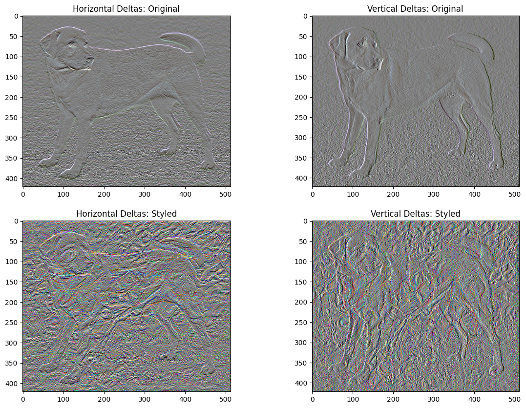
นี่แสดงให้เห็นว่าส่วนประกอบความถี่สูงเพิ่มขึ้นอย่างไร
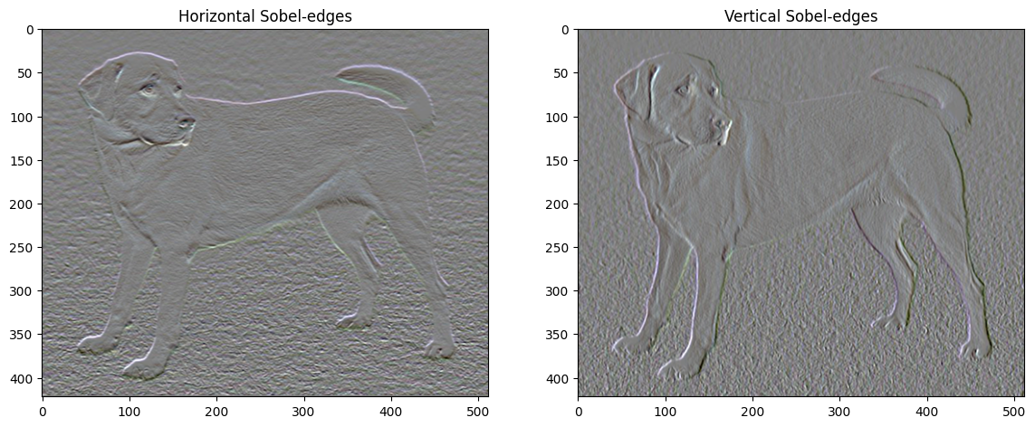
นอกจากนี้ ส่วนประกอบความถี่สูงนี้ยังเป็นเครื่องตรวจจับขอบอีกด้วย คุณสามารถรับเอาต์พุตที่คล้ายกันจากตัวตรวจจับขอบ Sobel ตัวอย่างเช่น:
plt.figure(figsize=(14, 10))

sobel = tf.image.sobel_edges(content_image)
plt.subplot(1, 2, 1)
imshow(clip_0_1(sobel[..., 0]/4+0.5), "Horizontal Sobel-edges")
plt.subplot(1, 2, 2)
imshow(clip_0_1(sobel[..., 1]/4+0.5), "Vertical Sobel-edges")
การสูญเสียการทำให้เป็นมาตรฐานที่เกี่ยวข้องกับสิ่งนี้คือผลรวมของกำลังสองของค่า:
def total_variation_loss(image):
  x_deltas, y_deltas = high_pass_x_y(image)
  return tf.reduce_sum(tf.abs(x_deltas)) + tf.reduce_sum(tf.abs(y_deltas))
total_variation_loss(image).numpy()
149402.94
ที่แสดงให้เห็นสิ่งที่มันทำ แต่ไม่จำเป็นต้องดำเนินการเอง TensorFlow มีการใช้งานมาตรฐาน:
tf.image.total_variation(image).numpy()
array([149402.94], dtype=float32)ตัวยึดตำแหน่ง42
เรียกใช้การเพิ่มประสิทธิภาพอีกครั้ง
เลือกน้ำหนักสำหรับ total_variation_loss :
total_variation_weight=30
ตอนนี้รวมไว้ในฟังก์ชัน train_step :
@tf.function()
def train_step(image):
  with tf.GradientTape() as tape:
    outputs = extractor(image)
    loss = style_content_loss(outputs)
    loss += total_variation_weight*tf.image.total_variation(image)

  grad = tape.gradient(loss, image)
  opt.apply_gradients([(grad, image)])
  image.assign(clip_0_1(image))
กำหนดค่าเริ่มต้นตัวแปรการปรับให้เหมาะสมใหม่:
image = tf.Variable(content_image)
และเรียกใช้การเพิ่มประสิทธิภาพ:
import time
start = time.time()

epochs = 10
steps_per_epoch = 100

step = 0
for n in range(epochs):
  for m in range(steps_per_epoch):
    step += 1
    train_step(image)
    print(".", end='', flush=True)
  display.clear_output(wait=True)
  display.display(tensor_to_image(image))
  print("Train step: {}".format(step))

end = time.time()
print("Total time: {:.1f}".format(end-start))
Train step: 1000
Total time: 22.4
สุดท้าย บันทึกผลลัพธ์:
file_name = 'stylized-image.png'
tensor_to_image(image).save(file_name)

try:
  from google.colab import files
except ImportError:
   pass
else:
  files.download(file_name)
เรียนรู้เพิ่มเติม
บทช่วยสอนนี้สาธิตอัลกอริทึมการถ่ายโอนสไตล์ดั้งเดิม สำหรับการประยุกต์ใช้การถ่ายโอนสไตล์อย่างง่าย โปรดดูบทช่วย สอน นี้เพื่อเรียนรู้เพิ่มเติมเกี่ยวกับวิธีใช้โมเดลการถ่ายโอนสไตล์รูปภาพที่กำหนดเองจาก TensorFlow Hub