
|
|
|
 View source on GitHub
|
|
This tutorial demonstrates how to preprocess audio files in the WAV format and build and train a basic automatic speech recognition (ASR) model for recognizing ten different words. You will use a portion of the Speech Commands dataset (Warden, 2018), which contains short (one-second or less) audio clips of commands, such as "down", "go", "left", "no", "right", "stop", "up" and "yes".
Real-world speech and audio recognition systems are complex. But, like image classification with the MNIST dataset, this tutorial should give you a basic understanding of the techniques involved.
Setup
Import necessary modules and dependencies. You'll be using tf.keras.utils.audio_dataset_from_directory (introduced in TensorFlow 2.10), which helps generate audio classification datasets from directories of .wav files. You'll also need seaborn for visualization in this tutorial.
pip install -U -q tensorflow tensorflow_datasetsimport os
import pathlib
import matplotlib.pyplot as plt
import numpy as np
import seaborn as sns
import tensorflow as tf
from tensorflow.keras import layers
from tensorflow.keras import models
from IPython import display
# Set the seed value for experiment reproducibility.
seed = 42
tf.random.set_seed(seed)
np.random.seed(seed)
2024-08-16 07:47:19.221318: E external/local_xla/xla/stream_executor/cuda/cuda_fft.cc:485] Unable to register cuFFT factory: Attempting to register factory for plugin cuFFT when one has already been registered
2024-08-16 07:47:19.242431: E external/local_xla/xla/stream_executor/cuda/cuda_dnn.cc:8454] Unable to register cuDNN factory: Attempting to register factory for plugin cuDNN when one has already been registered
2024-08-16 07:47:19.248832: E external/local_xla/xla/stream_executor/cuda/cuda_blas.cc:1452] Unable to register cuBLAS factory: Attempting to register factory for plugin cuBLAS when one has already been registered
Import the mini Speech Commands dataset
To save time with data loading, you will be working with a smaller version of the Speech Commands dataset. The original dataset consists of over 105,000 audio files in the WAV (Waveform) audio file format of people saying 35 different words. This data was collected by Google and released under a CC BY license.
Download and extract the mini_speech_commands.zip file containing the smaller Speech Commands datasets with tf.keras.utils.get_file:
DATASET_PATH = 'data/mini_speech_commands'

data_dir = pathlib.Path(DATASET_PATH)
if not data_dir.exists():
  tf.keras.utils.get_file(
      'mini_speech_commands.zip',
      origin="http://storage.googleapis.com/download.tensorflow.org/data/mini_speech_commands.zip",
      extract=True,
      cache_dir='.', cache_subdir='data')
Downloading data from http://storage.googleapis.com/download.tensorflow.org/data/mini_speech_commands.zip
182082353/182082353 ━━━━━━━━━━━━━━━━━━━━ 1s 0us/step
The dataset's audio clips are stored in eight folders corresponding to each speech command: no, yes, down, go, left, up, right, and stop:
commands = np.array(tf.io.gfile.listdir(str(data_dir)))
commands = commands[(commands != 'README.md') & (commands != '.DS_Store')]
print('Commands:', commands)
Commands: ['stop' 'up' 'left' 'yes' 'right' 'go' 'no' 'down']
Divided into directories this way, you can easily load the data using keras.utils.audio_dataset_from_directory.
The audio clips are 1 second or less at 16kHz. The output_sequence_length=16000 pads the short ones to exactly 1 second (and would trim longer ones) so that they can be easily batched.
train_ds, val_ds = tf.keras.utils.audio_dataset_from_directory(
    directory=data_dir,
    batch_size=64,
    validation_split=0.2,
    seed=0,
    output_sequence_length=16000,
    subset='both')

label_names = np.array(train_ds.class_names)
print()
print("label names:", label_names)
Found 8000 files belonging to 8 classes.
Using 6400 files for training.
Using 1600 files for validation.
WARNING: All log messages before absl::InitializeLog() is called are written to STDERR
I0000 00:00:1723794446.926622  244018 cuda_executor.cc:1015] successful NUMA node read from SysFS had negative value (-1), but there must be at least one NUMA node, so returning NUMA node zero. See more at https://github.com/torvalds/linux/blob/v6.0/Documentation/ABI/testing/sysfs-bus-pci#L344-L355
I0000 00:00:1723794446.930567  244018 cuda_executor.cc:1015] successful NUMA node read from SysFS had negative value (-1), but there must be at least one NUMA node, so returning NUMA node zero. See more at https://github.com/torvalds/linux/blob/v6.0/Documentation/ABI/testing/sysfs-bus-pci#L344-L355
I0000 00:00:1723794446.934298  244018 cuda_executor.cc:1015] successful NUMA node read from SysFS had negative value (-1), but there must be at least one NUMA node, so returning NUMA node zero. See more at https://github.com/torvalds/linux/blob/v6.0/Documentation/ABI/testing/sysfs-bus-pci#L344-L355
I0000 00:00:1723794446.938000  244018 cuda_executor.cc:1015] successful NUMA node read from SysFS had negative value (-1), but there must be at least one NUMA node, so returning NUMA node zero. See more at https://github.com/torvalds/linux/blob/v6.0/Documentation/ABI/testing/sysfs-bus-pci#L344-L355
I0000 00:00:1723794446.949122  244018 cuda_executor.cc:1015] successful NUMA node read from SysFS had negative value (-1), but there must be at least one NUMA node, so returning NUMA node zero. See more at https://github.com/torvalds/linux/blob/v6.0/Documentation/ABI/testing/sysfs-bus-pci#L344-L355
I0000 00:00:1723794446.952675  244018 cuda_executor.cc:1015] successful NUMA node read from SysFS had negative value (-1), but there must be at least one NUMA node, so returning NUMA node zero. See more at https://github.com/torvalds/linux/blob/v6.0/Documentation/ABI/testing/sysfs-bus-pci#L344-L355
I0000 00:00:1723794446.956214  244018 cuda_executor.cc:1015] successful NUMA node read from SysFS had negative value (-1), but there must be at least one NUMA node, so returning NUMA node zero. See more at https://github.com/torvalds/linux/blob/v6.0/Documentation/ABI/testing/sysfs-bus-pci#L344-L355
I0000 00:00:1723794446.959802  244018 cuda_executor.cc:1015] successful NUMA node read from SysFS had negative value (-1), but there must be at least one NUMA node, so returning NUMA node zero. See more at https://github.com/torvalds/linux/blob/v6.0/Documentation/ABI/testing/sysfs-bus-pci#L344-L355
I0000 00:00:1723794446.963275  244018 cuda_executor.cc:1015] successful NUMA node read from SysFS had negative value (-1), but there must be at least one NUMA node, so returning NUMA node zero. See more at https://github.com/torvalds/linux/blob/v6.0/Documentation/ABI/testing/sysfs-bus-pci#L344-L355
I0000 00:00:1723794446.966769  244018 cuda_executor.cc:1015] successful NUMA node read from SysFS had negative value (-1), but there must be at least one NUMA node, so returning NUMA node zero. See more at https://github.com/torvalds/linux/blob/v6.0/Documentation/ABI/testing/sysfs-bus-pci#L344-L355
I0000 00:00:1723794446.970214  244018 cuda_executor.cc:1015] successful NUMA node read from SysFS had negative value (-1), but there must be at least one NUMA node, so returning NUMA node zero. See more at https://github.com/torvalds/linux/blob/v6.0/Documentation/ABI/testing/sysfs-bus-pci#L344-L355
I0000 00:00:1723794446.973810  244018 cuda_executor.cc:1015] successful NUMA node read from SysFS had negative value (-1), but there must be at least one NUMA node, so returning NUMA node zero. See more at https://github.com/torvalds/linux/blob/v6.0/Documentation/ABI/testing/sysfs-bus-pci#L344-L355
I0000 00:00:1723794448.198791  244018 cuda_executor.cc:1015] successful NUMA node read from SysFS had negative value (-1), but there must be at least one NUMA node, so returning NUMA node zero. See more at https://github.com/torvalds/linux/blob/v6.0/Documentation/ABI/testing/sysfs-bus-pci#L344-L355
I0000 00:00:1723794448.200969  244018 cuda_executor.cc:1015] successful NUMA node read from SysFS had negative value (-1), but there must be at least one NUMA node, so returning NUMA node zero. See more at https://github.com/torvalds/linux/blob/v6.0/Documentation/ABI/testing/sysfs-bus-pci#L344-L355
I0000 00:00:1723794448.203188  244018 cuda_executor.cc:1015] successful NUMA node read from SysFS had negative value (-1), but there must be at least one NUMA node, so returning NUMA node zero. See more at https://github.com/torvalds/linux/blob/v6.0/Documentation/ABI/testing/sysfs-bus-pci#L344-L355
I0000 00:00:1723794448.205237  244018 cuda_executor.cc:1015] successful NUMA node read from SysFS had negative value (-1), but there must be at least one NUMA node, so returning NUMA node zero. See more at https://github.com/torvalds/linux/blob/v6.0/Documentation/ABI/testing/sysfs-bus-pci#L344-L355
I0000 00:00:1723794448.207299  244018 cuda_executor.cc:1015] successful NUMA node read from SysFS had negative value (-1), but there must be at least one NUMA node, so returning NUMA node zero. See more at https://github.com/torvalds/linux/blob/v6.0/Documentation/ABI/testing/sysfs-bus-pci#L344-L355
I0000 00:00:1723794448.209277  244018 cuda_executor.cc:1015] successful NUMA node read from SysFS had negative value (-1), but there must be at least one NUMA node, so returning NUMA node zero. See more at https://github.com/torvalds/linux/blob/v6.0/Documentation/ABI/testing/sysfs-bus-pci#L344-L355
I0000 00:00:1723794448.211246  244018 cuda_executor.cc:1015] successful NUMA node read from SysFS had negative value (-1), but there must be at least one NUMA node, so returning NUMA node zero. See more at https://github.com/torvalds/linux/blob/v6.0/Documentation/ABI/testing/sysfs-bus-pci#L344-L355
I0000 00:00:1723794448.213166  244018 cuda_executor.cc:1015] successful NUMA node read from SysFS had negative value (-1), but there must be at least one NUMA node, so returning NUMA node zero. See more at https://github.com/torvalds/linux/blob/v6.0/Documentation/ABI/testing/sysfs-bus-pci#L344-L355
I0000 00:00:1723794448.215121  244018 cuda_executor.cc:1015] successful NUMA node read from SysFS had negative value (-1), but there must be at least one NUMA node, so returning NUMA node zero. See more at https://github.com/torvalds/linux/blob/v6.0/Documentation/ABI/testing/sysfs-bus-pci#L344-L355
I0000 00:00:1723794448.217091  244018 cuda_executor.cc:1015] successful NUMA node read from SysFS had negative value (-1), but there must be at least one NUMA node, so returning NUMA node zero. See more at https://github.com/torvalds/linux/blob/v6.0/Documentation/ABI/testing/sysfs-bus-pci#L344-L355
I0000 00:00:1723794448.219066  244018 cuda_executor.cc:1015] successful NUMA node read from SysFS had negative value (-1), but there must be at least one NUMA node, so returning NUMA node zero. See more at https://github.com/torvalds/linux/blob/v6.0/Documentation/ABI/testing/sysfs-bus-pci#L344-L355
I0000 00:00:1723794448.220987  244018 cuda_executor.cc:1015] successful NUMA node read from SysFS had negative value (-1), but there must be at least one NUMA node, so returning NUMA node zero. See more at https://github.com/torvalds/linux/blob/v6.0/Documentation/ABI/testing/sysfs-bus-pci#L344-L355
I0000 00:00:1723794448.260509  244018 cuda_executor.cc:1015] successful NUMA node read from SysFS had negative value (-1), but there must be at least one NUMA node, so returning NUMA node zero. See more at https://github.com/torvalds/linux/blob/v6.0/Documentation/ABI/testing/sysfs-bus-pci#L344-L355
I0000 00:00:1723794448.262572  244018 cuda_executor.cc:1015] successful NUMA node read from SysFS had negative value (-1), but there must be at least one NUMA node, so returning NUMA node zero. See more at https://github.com/torvalds/linux/blob/v6.0/Documentation/ABI/testing/sysfs-bus-pci#L344-L355
I0000 00:00:1723794448.264601  244018 cuda_executor.cc:1015] successful NUMA node read from SysFS had negative value (-1), but there must be at least one NUMA node, so returning NUMA node zero. See more at https://github.com/torvalds/linux/blob/v6.0/Documentation/ABI/testing/sysfs-bus-pci#L344-L355
I0000 00:00:1723794448.266575  244018 cuda_executor.cc:1015] successful NUMA node read from SysFS had negative value (-1), but there must be at least one NUMA node, so returning NUMA node zero. See more at https://github.com/torvalds/linux/blob/v6.0/Documentation/ABI/testing/sysfs-bus-pci#L344-L355
I0000 00:00:1723794448.268552  244018 cuda_executor.cc:1015] successful NUMA node read from SysFS had negative value (-1), but there must be at least one NUMA node, so returning NUMA node zero. See more at https://github.com/torvalds/linux/blob/v6.0/Documentation/ABI/testing/sysfs-bus-pci#L344-L355
I0000 00:00:1723794448.270529  244018 cuda_executor.cc:1015] successful NUMA node read from SysFS had negative value (-1), but there must be at least one NUMA node, so returning NUMA node zero. See more at https://github.com/torvalds/linux/blob/v6.0/Documentation/ABI/testing/sysfs-bus-pci#L344-L355
I0000 00:00:1723794448.272511  244018 cuda_executor.cc:1015] successful NUMA node read from SysFS had negative value (-1), but there must be at least one NUMA node, so returning NUMA node zero. See more at https://github.com/torvalds/linux/blob/v6.0/Documentation/ABI/testing/sysfs-bus-pci#L344-L355
I0000 00:00:1723794448.274547  244018 cuda_executor.cc:1015] successful NUMA node read from SysFS had negative value (-1), but there must be at least one NUMA node, so returning NUMA node zero. See more at https://github.com/torvalds/linux/blob/v6.0/Documentation/ABI/testing/sysfs-bus-pci#L344-L355
I0000 00:00:1723794448.276566  244018 cuda_executor.cc:1015] successful NUMA node read from SysFS had negative value (-1), but there must be at least one NUMA node, so returning NUMA node zero. See more at https://github.com/torvalds/linux/blob/v6.0/Documentation/ABI/testing/sysfs-bus-pci#L344-L355
I0000 00:00:1723794448.279079  244018 cuda_executor.cc:1015] successful NUMA node read from SysFS had negative value (-1), but there must be at least one NUMA node, so returning NUMA node zero. See more at https://github.com/torvalds/linux/blob/v6.0/Documentation/ABI/testing/sysfs-bus-pci#L344-L355
I0000 00:00:1723794448.281515  244018 cuda_executor.cc:1015] successful NUMA node read from SysFS had negative value (-1), but there must be at least one NUMA node, so returning NUMA node zero. See more at https://github.com/torvalds/linux/blob/v6.0/Documentation/ABI/testing/sysfs-bus-pci#L344-L355
I0000 00:00:1723794448.283888  244018 cuda_executor.cc:1015] successful NUMA node read from SysFS had negative value (-1), but there must be at least one NUMA node, so returning NUMA node zero. See more at https://github.com/torvalds/linux/blob/v6.0/Documentation/ABI/testing/sysfs-bus-pci#L344-L355
label names: ['down' 'go' 'left' 'no' 'right' 'stop' 'up' 'yes']
The dataset now contains batches of audio clips and integer labels. The audio clips have a shape of (batch, samples, channels).
train_ds.element_spec
(TensorSpec(shape=(None, 16000, None), dtype=tf.float32, name=None),
 TensorSpec(shape=(None,), dtype=tf.int32, name=None))
This dataset only contains single channel audio, so use the tf.squeeze function to drop the extra axis:
def squeeze(audio, labels):
  audio = tf.squeeze(audio, axis=-1)
  return audio, labels

train_ds = train_ds.map(squeeze, tf.data.AUTOTUNE)
val_ds = val_ds.map(squeeze, tf.data.AUTOTUNE)
The utils.audio_dataset_from_directory function only returns up to two splits. It's a good idea to keep a test set separate from your validation set.
Ideally you'd keep it in a separate directory, but in this case you can use Dataset.shard to split the validation set into two halves. Note that iterating over any shard will load all the data, and only keep its fraction.
test_ds = val_ds.shard(num_shards=2, index=0)
val_ds = val_ds.shard(num_shards=2, index=1)
for example_audio, example_labels in train_ds.take(1):
  print(example_audio.shape)
  print(example_labels.shape)
(64, 16000)
(64,)
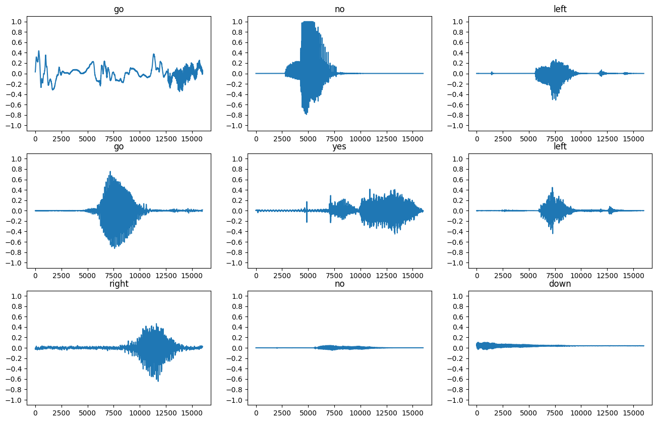
Let's plot a few audio waveforms:
label_names[[1,1,3,0]]
array(['go', 'go', 'no', 'down'], dtype='<U5')
plt.figure(figsize=(16, 10))
rows = 3
cols = 3
n = rows * cols
for i in range(n):
  plt.subplot(rows, cols, i+1)
  audio_signal = example_audio[i]
  plt.plot(audio_signal)
  plt.title(label_names[example_labels[i]])
  plt.yticks(np.arange(-1.2, 1.2, 0.2))
  plt.ylim([-1.1, 1.1])
Convert waveforms to spectrograms
The waveforms in the dataset are represented in the time domain. Next, you'll transform the waveforms from the time-domain signals into the time-frequency-domain signals by computing the short-time Fourier transform (STFT) to convert the waveforms to as spectrograms, which show frequency changes over time and can be represented as 2D images. You will feed the spectrogram images into your neural network to train the model.
A Fourier transform (tf.signal.fft) converts a signal to its component frequencies, but loses all time information. In comparison, STFT (tf.signal.stft) splits the signal into windows of time and runs a Fourier transform on each window, preserving some time information, and returning a 2D tensor that you can run standard convolutions on.
Create a utility function for converting waveforms to spectrograms:
- The waveforms need to be of the same length, so that when you convert them to spectrograms, the results have similar dimensions. This can be done by simply zero-padding the audio clips that are shorter than one second (using
tf.zeros). - When calling
tf.signal.stft, choose theframe_lengthandframe_stepparameters such that the generated spectrogram "image" is almost square. For more information on the STFT parameters choice, refer to this Coursera video on audio signal processing and STFT. - The STFT produces an array of complex numbers representing magnitude and phase. However, in this tutorial you'll only use the magnitude, which you can derive by applying
tf.abson the output oftf.signal.stft.
def get_spectrogram(waveform):
  # Convert the waveform to a spectrogram via a STFT.
  spectrogram = tf.signal.stft(
      waveform, frame_length=255, frame_step=128)
  # Obtain the magnitude of the STFT.
  spectrogram = tf.abs(spectrogram)
  # Add a `channels` dimension, so that the spectrogram can be used
  # as image-like input data with convolution layers (which expect
  # shape (`batch_size`, `height`, `width`, `channels`).
  spectrogram = spectrogram[..., tf.newaxis]
  return spectrogram
Next, start exploring the data. Print the shapes of one example's tensorized waveform and the corresponding spectrogram, and play the original audio:
for i in range(3):
  label = label_names[example_labels[i]]
  waveform = example_audio[i]
  spectrogram = get_spectrogram(waveform)

  print('Label:', label)
  print('Waveform shape:', waveform.shape)
  print('Spectrogram shape:', spectrogram.shape)
  print('Audio playback')
  display.display(display.Audio(waveform, rate=16000))
Label: go
Waveform shape: (16000,)
Spectrogram shape: (124, 129, 1)
Audio playback
Label: no
Waveform shape: (16000,)
Spectrogram shape: (124, 129, 1)
Audio playback
Label: left
Waveform shape: (16000,)
Spectrogram shape: (124, 129, 1)
Audio playback
Now, define a function for displaying a spectrogram:
def plot_spectrogram(spectrogram, ax):
  if len(spectrogram.shape) > 2:
    assert len(spectrogram.shape) == 3
    spectrogram = np.squeeze(spectrogram, axis=-1)
  # Convert the frequencies to log scale and transpose, so that the time is
  # represented on the x-axis (columns).
  # Add an epsilon to avoid taking a log of zero.
  log_spec = np.log(spectrogram.T + np.finfo(float).eps)
  height = log_spec.shape[0]
  width = log_spec.shape[1]
  X = np.linspace(0, np.size(spectrogram), num=width, dtype=int)
  Y = range(height)
  ax.pcolormesh(X, Y, log_spec)
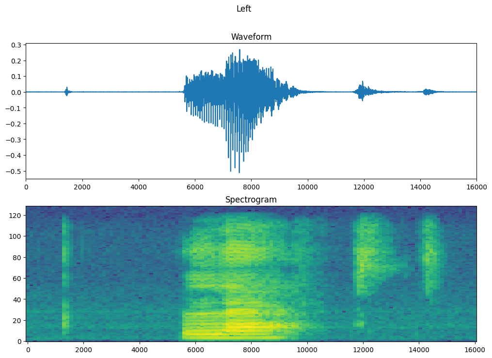
Plot the example's waveform over time and the corresponding spectrogram (frequencies over time):
fig, axes = plt.subplots(2, figsize=(12, 8))
timescale = np.arange(waveform.shape[0])
axes[0].plot(timescale, waveform.numpy())
axes[0].set_title('Waveform')
axes[0].set_xlim([0, 16000])

plot_spectrogram(spectrogram.numpy(), axes[1])
axes[1].set_title('Spectrogram')
plt.suptitle(label.title())
plt.show()
Now, create spectrogram datasets from the audio datasets:
def make_spec_ds(ds):
  return ds.map(
      map_func=lambda audio,label: (get_spectrogram(audio), label),
      num_parallel_calls=tf.data.AUTOTUNE)
train_spectrogram_ds = make_spec_ds(train_ds)
val_spectrogram_ds = make_spec_ds(val_ds)
test_spectrogram_ds = make_spec_ds(test_ds)
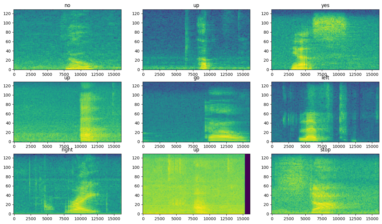
Examine the spectrograms for different examples of the dataset:
for example_spectrograms, example_spect_labels in train_spectrogram_ds.take(1):
  break
rows = 3
cols = 3
n = rows*cols
fig, axes = plt.subplots(rows, cols, figsize=(16, 9))

for i in range(n):
    r = i // cols
    c = i % cols
    ax = axes[r][c]
    plot_spectrogram(example_spectrograms[i].numpy(), ax)
    ax.set_title(label_names[example_spect_labels[i].numpy()])

plt.show()
Build and train the model
Add Dataset.cache and Dataset.prefetch operations to reduce read latency while training the model:
train_spectrogram_ds = train_spectrogram_ds.cache().shuffle(10000).prefetch(tf.data.AUTOTUNE)
val_spectrogram_ds = val_spectrogram_ds.cache().prefetch(tf.data.AUTOTUNE)
test_spectrogram_ds = test_spectrogram_ds.cache().prefetch(tf.data.AUTOTUNE)
For the model, you'll use a simple convolutional neural network (CNN), since you have transformed the audio files into spectrogram images.
Your tf.keras.Sequential model will use the following Keras preprocessing layers:
tf.keras.layers.Resizing: to downsample the input to enable the model to train faster.tf.keras.layers.Normalization: to normalize each pixel in the image based on its mean and standard deviation.
For the Normalization layer, its adapt method would first need to be called on the training data in order to compute aggregate statistics (that is, the mean and the standard deviation).
input_shape = example_spectrograms.shape[1:]
print('Input shape:', input_shape)
num_labels = len(label_names)

# Instantiate the `tf.keras.layers.Normalization` layer.
norm_layer = layers.Normalization()
# Fit the state of the layer to the spectrograms
# with `Normalization.adapt`.
norm_layer.adapt(data=train_spectrogram_ds.map(map_func=lambda spec, label: spec))

model = models.Sequential([
    layers.Input(shape=input_shape),
    # Downsample the input.
    layers.Resizing(32, 32),
    # Normalize.
    norm_layer,
    layers.Conv2D(32, 3, activation='relu'),
    layers.Conv2D(64, 3, activation='relu'),
    layers.MaxPooling2D(),
    layers.Dropout(0.25),
    layers.Flatten(),
    layers.Dense(128, activation='relu'),
    layers.Dropout(0.5),
    layers.Dense(num_labels),
])

model.summary()
Input shape: (124, 129, 1)
Configure the Keras model with the Adam optimizer and the cross-entropy loss:
model.compile(
    optimizer=tf.keras.optimizers.Adam(),
    loss=tf.keras.losses.SparseCategoricalCrossentropy(from_logits=True),
    metrics=['accuracy'],
)
Train the model over 10 epochs for demonstration purposes:
EPOCHS = 10
history = model.fit(
    train_spectrogram_ds,
    validation_data=val_spectrogram_ds,
    epochs=EPOCHS,
    callbacks=tf.keras.callbacks.EarlyStopping(verbose=1, patience=2),
)
Epoch 1/10
WARNING: All log messages before absl::InitializeLog() is called are written to STDERR
I0000 00:00:1723794456.367614  244224 service.cc:146] XLA service 0x7f52d4004720 initialized for platform CUDA (this does not guarantee that XLA will be used). Devices:
I0000 00:00:1723794456.367645  244224 service.cc:154]   StreamExecutor device (0): Tesla T4, Compute Capability 7.5
I0000 00:00:1723794456.367649  244224 service.cc:154]   StreamExecutor device (1): Tesla T4, Compute Capability 7.5
I0000 00:00:1723794456.367651  244224 service.cc:154]   StreamExecutor device (2): Tesla T4, Compute Capability 7.5
I0000 00:00:1723794456.367654  244224 service.cc:154]   StreamExecutor device (3): Tesla T4, Compute Capability 7.5
28/100 ━━━━━━━━━━━━━━━━━━━━ 0s 6ms/step - accuracy: 0.1942 - loss: 2.0681
I0000 00:00:1723794458.966081  244224 device_compiler.h:188] Compiled cluster using XLA!  This line is logged at most once for the lifetime of the process.
100/100 ━━━━━━━━━━━━━━━━━━━━ 5s 16ms/step - accuracy: 0.2918 - loss: 1.9072 - val_accuracy: 0.5990 - val_loss: 1.3176
Epoch 2/10
100/100 ━━━━━━━━━━━━━━━━━━━━ 1s 6ms/step - accuracy: 0.5629 - loss: 1.2572 - val_accuracy: 0.7240 - val_loss: 0.9291
Epoch 3/10
100/100 ━━━━━━━━━━━━━━━━━━━━ 1s 6ms/step - accuracy: 0.6770 - loss: 0.9247 - val_accuracy: 0.7943 - val_loss: 0.7514
Epoch 4/10
100/100 ━━━━━━━━━━━━━━━━━━━━ 1s 6ms/step - accuracy: 0.7396 - loss: 0.7337 - val_accuracy: 0.8021 - val_loss: 0.6488
Epoch 5/10
100/100 ━━━━━━━━━━━━━━━━━━━━ 1s 6ms/step - accuracy: 0.7819 - loss: 0.6244 - val_accuracy: 0.8346 - val_loss: 0.6065
Epoch 6/10
100/100 ━━━━━━━━━━━━━━━━━━━━ 1s 6ms/step - accuracy: 0.8053 - loss: 0.5551 - val_accuracy: 0.8229 - val_loss: 0.5916
Epoch 7/10
100/100 ━━━━━━━━━━━━━━━━━━━━ 1s 6ms/step - accuracy: 0.8278 - loss: 0.4883 - val_accuracy: 0.8398 - val_loss: 0.5661
Epoch 8/10
100/100 ━━━━━━━━━━━━━━━━━━━━ 1s 6ms/step - accuracy: 0.8447 - loss: 0.4542 - val_accuracy: 0.8320 - val_loss: 0.5266
Epoch 9/10
100/100 ━━━━━━━━━━━━━━━━━━━━ 1s 6ms/step - accuracy: 0.8684 - loss: 0.3811 - val_accuracy: 0.8542 - val_loss: 0.5053
Epoch 10/10
100/100 ━━━━━━━━━━━━━━━━━━━━ 1s 6ms/step - accuracy: 0.8802 - loss: 0.3423 - val_accuracy: 0.8451 - val_loss: 0.4709
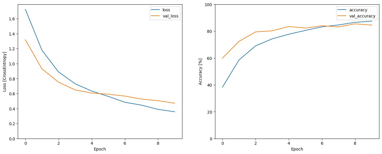
Let's plot the training and validation loss curves to check how your model has improved during training:
metrics = history.history
plt.figure(figsize=(16,6))
plt.subplot(1,2,1)
plt.plot(history.epoch, metrics['loss'], metrics['val_loss'])
plt.legend(['loss', 'val_loss'])
plt.ylim([0, max(plt.ylim())])
plt.xlabel('Epoch')
plt.ylabel('Loss [CrossEntropy]')

plt.subplot(1,2,2)
plt.plot(history.epoch, 100*np.array(metrics['accuracy']), 100*np.array(metrics['val_accuracy']))
plt.legend(['accuracy', 'val_accuracy'])
plt.ylim([0, 100])
plt.xlabel('Epoch')
plt.ylabel('Accuracy [%]')
Text(0, 0.5, 'Accuracy [%]')
Evaluate the model performance
Run the model on the test set and check the model's performance:
model.evaluate(test_spectrogram_ds, return_dict=True)
13/13 ━━━━━━━━━━━━━━━━━━━━ 0s 4ms/step - accuracy: 0.8255 - loss: 0.5090
{'accuracy': 0.832932710647583, 'loss': 0.5049060583114624}
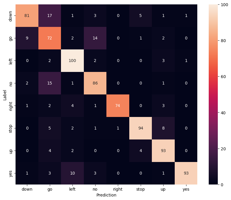
Display a confusion matrix
Use a confusion matrix to check how well the model did classifying each of the commands in the test set:
y_pred = model.predict(test_spectrogram_ds)
13/13 ━━━━━━━━━━━━━━━━━━━━ 0s 3ms/step
y_pred = tf.argmax(y_pred, axis=1)
y_true = tf.concat(list(test_spectrogram_ds.map(lambda s,lab: lab)), axis=0)
confusion_mtx = tf.math.confusion_matrix(y_true, y_pred)
plt.figure(figsize=(10, 8))
sns.heatmap(confusion_mtx,
            xticklabels=label_names,
            yticklabels=label_names,
            annot=True, fmt='g')
plt.xlabel('Prediction')
plt.ylabel('Label')
plt.show()
Run inference on an audio file
Finally, verify the model's prediction output using an input audio file of someone saying "no". How well does your model perform?
x = data_dir/'no/01bb6a2a_nohash_0.wav'
x = tf.io.read_file(str(x))
x, sample_rate = tf.audio.decode_wav(x, desired_channels=1, desired_samples=16000,)
x = tf.squeeze(x, axis=-1)
waveform = x
x = get_spectrogram(x)
x = x[tf.newaxis,...]

prediction = model(x)
x_labels = ['no', 'yes', 'down', 'go', 'left', 'up', 'right', 'stop']
plt.bar(x_labels, tf.nn.softmax(prediction[0]))
plt.title('No')
plt.show()

display.display(display.Audio(waveform, rate=16000))
W0000 00:00:1723794468.163578  244018 gpu_timer.cc:114] Skipping the delay kernel, measurement accuracy will be reduced
W0000 00:00:1723794468.181379  244018 gpu_timer.cc:114] Skipping the delay kernel, measurement accuracy will be reduced
W0000 00:00:1723794468.182527  244018 gpu_timer.cc:114] Skipping the delay kernel, measurement accuracy will be reduced
W0000 00:00:1723794468.183650  244018 gpu_timer.cc:114] Skipping the delay kernel, measurement accuracy will be reduced
W0000 00:00:1723794468.184778  244018 gpu_timer.cc:114] Skipping the delay kernel, measurement accuracy will be reduced
W0000 00:00:1723794468.185904  244018 gpu_timer.cc:114] Skipping the delay kernel, measurement accuracy will be reduced
W0000 00:00:1723794468.187040  244018 gpu_timer.cc:114] Skipping the delay kernel, measurement accuracy will be reduced
W0000 00:00:1723794468.188192  244018 gpu_timer.cc:114] Skipping the delay kernel, measurement accuracy will be reduced
W0000 00:00:1723794468.189325  244018 gpu_timer.cc:114] Skipping the delay kernel, measurement accuracy will be reduced
W0000 00:00:1723794468.190479  244018 gpu_timer.cc:114] Skipping the delay kernel, measurement accuracy will be reduced
W0000 00:00:1723794468.191596  244018 gpu_timer.cc:114] Skipping the delay kernel, measurement accuracy will be reduced
W0000 00:00:1723794468.192715  244018 gpu_timer.cc:114] Skipping the delay kernel, measurement accuracy will be reduced
W0000 00:00:1723794468.193885  244018 gpu_timer.cc:114] Skipping the delay kernel, measurement accuracy will be reduced
W0000 00:00:1723794468.195045  244018 gpu_timer.cc:114] Skipping the delay kernel, measurement accuracy will be reduced
W0000 00:00:1723794468.196165  244018 gpu_timer.cc:114] Skipping the delay kernel, measurement accuracy will be reduced
W0000 00:00:1723794468.197279  244018 gpu_timer.cc:114] Skipping the delay kernel, measurement accuracy will be reduced
W0000 00:00:1723794468.198522  244018 gpu_timer.cc:114] Skipping the delay kernel, measurement accuracy will be reduced
W0000 00:00:1723794468.275515  244018 gpu_timer.cc:114] Skipping the delay kernel, measurement accuracy will be reduced
W0000 00:00:1723794468.276725  244018 gpu_timer.cc:114] Skipping the delay kernel, measurement accuracy will be reduced
W0000 00:00:1723794468.277901  244018 gpu_timer.cc:114] Skipping the delay kernel, measurement accuracy will be reduced
W0000 00:00:1723794468.279116  244018 gpu_timer.cc:114] Skipping the delay kernel, measurement accuracy will be reduced
W0000 00:00:1723794468.280313  244018 gpu_timer.cc:114] Skipping the delay kernel, measurement accuracy will be reduced
W0000 00:00:1723794468.281515  244018 gpu_timer.cc:114] Skipping the delay kernel, measurement accuracy will be reduced
W0000 00:00:1723794468.282728  244018 gpu_timer.cc:114] Skipping the delay kernel, measurement accuracy will be reduced
W0000 00:00:1723794468.283930  244018 gpu_timer.cc:114] Skipping the delay kernel, measurement accuracy will be reduced
W0000 00:00:1723794468.285150  244018 gpu_timer.cc:114] Skipping the delay kernel, measurement accuracy will be reduced
W0000 00:00:1723794468.286374  244018 gpu_timer.cc:114] Skipping the delay kernel, measurement accuracy will be reduced
W0000 00:00:1723794468.287601  244018 gpu_timer.cc:114] Skipping the delay kernel, measurement accuracy will be reduced
W0000 00:00:1723794468.288818  244018 gpu_timer.cc:114] Skipping the delay kernel, measurement accuracy will be reduced
W0000 00:00:1723794468.290043  244018 gpu_timer.cc:114] Skipping the delay kernel, measurement accuracy will be reduced
W0000 00:00:1723794468.291301  244018 gpu_timer.cc:114] Skipping the delay kernel, measurement accuracy will be reduced
W0000 00:00:1723794468.292557  244018 gpu_timer.cc:114] Skipping the delay kernel, measurement accuracy will be reduced
W0000 00:00:1723794468.293707  244018 gpu_timer.cc:114] Skipping the delay kernel, measurement accuracy will be reduced
W0000 00:00:1723794468.295302  244018 gpu_timer.cc:114] Skipping the delay kernel, measurement accuracy will be reduced
W0000 00:00:1723794468.301178  244018 gpu_timer.cc:114] Skipping the delay kernel, measurement accuracy will be reduced
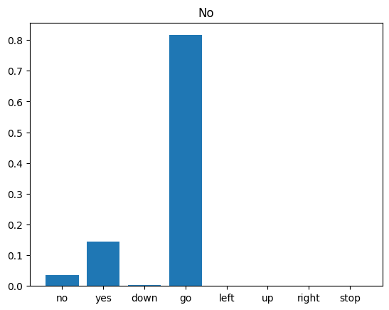
As the output suggests, your model should have recognized the audio command as "no".
Export the model with preprocessing
The model's not very easy to use if you have to apply those preprocessing steps before passing data to the model for inference. So build an end-to-end version:
class ExportModel(tf.Module):
  def __init__(self, model):
    self.model = model

    # Accept either a string-filename or a batch of waveforms.
    # YOu could add additional signatures for a single wave, or a ragged-batch.
    self.__call__.get_concrete_function(
        x=tf.TensorSpec(shape=(), dtype=tf.string))
    self.__call__.get_concrete_function(
       x=tf.TensorSpec(shape=[None, 16000], dtype=tf.float32))


  @tf.function
  def __call__(self, x):
    # If they pass a string, load the file and decode it.
    if x.dtype == tf.string:
      x = tf.io.read_file(x)
      x, _ = tf.audio.decode_wav(x, desired_channels=1, desired_samples=16000,)
      x = tf.squeeze(x, axis=-1)
      x = x[tf.newaxis, :]

    x = get_spectrogram(x)
    result = self.model(x, training=False)

    class_ids = tf.argmax(result, axis=-1)
    class_names = tf.gather(label_names, class_ids)
    return {'predictions':result,
            'class_ids': class_ids,
            'class_names': class_names}
Test run the "export" model:
export = ExportModel(model)
export(tf.constant(str(data_dir/'no/01bb6a2a_nohash_0.wav')))
{'predictions': <tf.Tensor: shape=(1, 8), dtype=float32, numpy=
 array([[ 1.0958828,  2.526922 , -1.8349309,  4.2553926, -4.2595496,
         -2.5386834, -3.6104631, -2.295511 ]], dtype=float32)>,
 'class_ids': <tf.Tensor: shape=(1,), dtype=int64, numpy=array([3])>,
 'class_names': <tf.Tensor: shape=(1,), dtype=string, numpy=array([b'no'], dtype=object)>}
Save and reload the model, the reloaded model gives identical output:
tf.saved_model.save(export, "saved")
imported = tf.saved_model.load("saved")
imported(waveform[tf.newaxis, :])
INFO:tensorflow:Assets written to: saved/assets
INFO:tensorflow:Assets written to: saved/assets
{'predictions': <tf.Tensor: shape=(1, 8), dtype=float32, numpy=
 array([[ 1.0958828,  2.526922 , -1.8349309,  4.2553926, -4.2595496,
         -2.5386834, -3.6104631, -2.295511 ]], dtype=float32)>,
 'class_ids': <tf.Tensor: shape=(1,), dtype=int64, numpy=array([3])>,
 'class_names': <tf.Tensor: shape=(1,), dtype=string, numpy=array([b'no'], dtype=object)>}
Next steps
This tutorial demonstrated how to carry out simple audio classification/automatic speech recognition using a convolutional neural network with TensorFlow and Python. To learn more, consider the following resources:
- The Sound classification with YAMNet tutorial shows how to use transfer learning for audio classification.
- The notebooks from Kaggle's TensorFlow speech recognition challenge.
- The TensorFlow.js - Audio recognition using transfer learning codelab teaches how to build your own interactive web app for audio classification.
- A tutorial on deep learning for music information retrieval (Choi et al., 2017) on arXiv.
- TensorFlow also has additional support for audio data preparation and augmentation to help with your own audio-based projects.
- Consider using the librosa library for music and audio analysis.