3D 畳み込みニューラルネットワークによる動画分類

TensorFlow.org で表示

Google Colab で実行

GitHub でソースを表示

ノートブックをダウンロード

This tutorial demonstrates training a 3D convolutional neural network (CNN) for video classification using the UCF101 action recognition dataset. A 3D CNN uses a three-dimensional filter to perform convolutions. The kernel is able to slide in three directions, whereas in a 2D CNN it can slide in two dimensions. The model is based on the work published in A Closer Look at Spatiotemporal Convolutions for Action Recognition by D. Tran et al. (2017). In this tutorial, you will:

• 入力パイプラインを構築する
• Keras Functional API を使って残差接続を伴う 3D 畳み込みニューラルネットワークモデルを構築する
• モデルをトレーニングする
• モデルを評価してテストする

This video classification tutorial is the second part in a series of TensorFlow video tutorials. Here are the other three tutorials:

• Load video data: This tutorial explains much of the code used in this document.
• MoViNet for streaming action recognition: Get familiar with the MoViNet models that are available on TF Hub.
• Transfer learning for video classification with MoViNet: This tutorial explains how to use a pre-trained video classification model trained on a different dataset with the UCF-101 dataset.

セットアップ

まず、ZIP ファイルの内容を検査するための remotezip、進捗バーを使用するための tqdm、動画ファイルを処理するための OpenCV、より複雑なテンソル演算を実行するための einops、Jupyter ノートブックにデータを埋め込むための tensorflow_docs を含む、必要なライブラリのインストールとインポートを行います。

注意: このチュートリアルは、TensorFlow 2.10 を使って実行します。TensorFlow 2.10 より後のバージョンでは、正しく実行しない可能性があります。

pip install remotezip tqdm opencv-python einops

import tqdm
import random
import pathlib
import itertools
import collections

import cv2
import einops
import numpy as np
import remotezip as rz
import seaborn as sns
import matplotlib.pyplot as plt

import tensorflow as tf
import keras
from keras import layers

2024-01-11 19:24:24.449591: E external/local_xla/xla/stream_executor/cuda/cuda_dnn.cc:9261] Unable to register cuDNN factory: Attempting to register factory for plugin cuDNN when one has already been registered
2024-01-11 19:24:24.449639: E external/local_xla/xla/stream_executor/cuda/cuda_fft.cc:607] Unable to register cuFFT factory: Attempting to register factory for plugin cuFFT when one has already been registered
2024-01-11 19:24:24.451390: E external/local_xla/xla/stream_executor/cuda/cuda_blas.cc:1515] Unable to register cuBLAS factory: Attempting to register factory for plugin cuBLAS when one has already been registered

動画データを読み込んで前処理する

以下の非表示セルは、UCF-101 データセットからデータスライスをダウンロードして tf.data.Dataset に読み込むヘルパー関数を定義します。具体的な前処理手順については、動画データの読み込みチュートリアルをご覧ください。このコードを手順を追ってより詳しく説明しています。

ここでは、非表示ブロックの最後にある FrameGenerator クラスが最も重要なユーティリティです。TensorFlow データパイプラインにデータをフィードでキルイテレート可能なオブジェクトを作成します。特に、このクラスには、エンコードされたラベルとともに動画フレームを読み込む Python ジェネレータが含まれます。このジェネレータ（__call__）関数は、frames_from_video_file とフレームセットに関連するラベルのワンホットエンコードのベクトルを生成します。

def list_files_per_class(zip_url):
  """
    List the files in each class of the dataset given the zip URL.

    Args:
      zip_url: URL from which the files can be unzipped. 

    Return:
      files: List of files in each of the classes.
  """
  files = []
  with rz.RemoteZip(URL) as zip:
    for zip_info in zip.infolist():
      files.append(zip_info.filename)
  return files

def get_class(fname):
  """
    Retrieve the name of the class given a filename.

    Args:
      fname: Name of the file in the UCF101 dataset.

    Return:
      Class that the file belongs to.
  """
  return fname.split('_')[-3]

def get_files_per_class(files):
  """
    Retrieve the files that belong to each class. 

    Args:
      files: List of files in the dataset.

    Return:
      Dictionary of class names (key) and files (values).
  """
  files_for_class = collections.defaultdict(list)
  for fname in files:
    class_name = get_class(fname)
    files_for_class[class_name].append(fname)
  return files_for_class

def download_from_zip(zip_url, to_dir, file_names):
  """
    Download the contents of the zip file from the zip URL.

    Args:
      zip_url: Zip URL containing data.
      to_dir: Directory to download data to.
      file_names: Names of files to download.
  """
  with rz.RemoteZip(zip_url) as zip:
    for fn in tqdm.tqdm(file_names):
      class_name = get_class(fn)
      zip.extract(fn, str(to_dir / class_name))
      unzipped_file = to_dir / class_name / fn

      fn = pathlib.Path(fn).parts[-1]
      output_file = to_dir / class_name / fn
      unzipped_file.rename(output_file,)

def split_class_lists(files_for_class, count):
  """
    Returns the list of files belonging to a subset of data as well as the remainder of
    files that need to be downloaded.

    Args:
      files_for_class: Files belonging to a particular class of data.
      count: Number of files to download.

    Return:
      split_files: Files belonging to the subset of data.
      remainder: Dictionary of the remainder of files that need to be downloaded.
  """
  split_files = []
  remainder = {}
  for cls in files_for_class:
    split_files.extend(files_for_class[cls][:count])
    remainder[cls] = files_for_class[cls][count:]
  return split_files, remainder

def download_ufc_101_subset(zip_url, num_classes, splits, download_dir):
  """
    Download a subset of the UFC101 dataset and split them into various parts, such as
    training, validation, and test. 

    Args:
      zip_url: Zip URL containing data.
      num_classes: Number of labels.
      splits: Dictionary specifying the training, validation, test, etc. (key) division of data 
              (value is number of files per split).
      download_dir: Directory to download data to.

    Return:
      dir: Posix path of the resulting directories containing the splits of data.
  """
  files = list_files_per_class(zip_url)
  for f in files:
    tokens = f.split('/')
    if len(tokens) <= 2:
      files.remove(f) # Remove that item from the list if it does not have a filename

  files_for_class = get_files_per_class(files)

  classes = list(files_for_class.keys())[:num_classes]

  for cls in classes:
    new_files_for_class = files_for_class[cls]
    random.shuffle(new_files_for_class)
    files_for_class[cls] = new_files_for_class

  # Only use the number of classes you want in the dictionary
  files_for_class = {x: files_for_class[x] for x in list(files_for_class)[:num_classes]}

  dirs = {}
  for split_name, split_count in splits.items():
    print(split_name, ":")
    split_dir = download_dir / split_name
    split_files, files_for_class = split_class_lists(files_for_class, split_count)
    download_from_zip(zip_url, split_dir, split_files)
    dirs[split_name] = split_dir

  return dirs

def format_frames(frame, output_size):
  """
    Pad and resize an image from a video.

    Args:
      frame: Image that needs to resized and padded. 
      output_size: Pixel size of the output frame image.

    Return:
      Formatted frame with padding of specified output size.
  """
  frame = tf.image.convert_image_dtype(frame, tf.float32)
  frame = tf.image.resize_with_pad(frame, *output_size)
  return frame

def frames_from_video_file(video_path, n_frames, output_size = (224,224), frame_step = 15):
  """
    Creates frames from each video file present for each category.

    Args:
      video_path: File path to the video.
      n_frames: Number of frames to be created per video file.
      output_size: Pixel size of the output frame image.

    Return:
      An NumPy array of frames in the shape of (n_frames, height, width, channels).
  """
  # Read each video frame by frame
  result = []
  src = cv2.VideoCapture(str(video_path))  

  video_length = src.get(cv2.CAP_PROP_FRAME_COUNT)

  need_length = 1 + (n_frames - 1) * frame_step

  if need_length > video_length:
    start = 0
  else:
    max_start = video_length - need_length
    start = random.randint(0, max_start + 1)

  src.set(cv2.CAP_PROP_POS_FRAMES, start)
  # ret is a boolean indicating whether read was successful, frame is the image itself
  ret, frame = src.read()
  result.append(format_frames(frame, output_size))

  for _ in range(n_frames - 1):
    for _ in range(frame_step):
      ret, frame = src.read()
    if ret:
      frame = format_frames(frame, output_size)
      result.append(frame)
    else:
      result.append(np.zeros_like(result[0]))
  src.release()
  result = np.array(result)[..., [2, 1, 0]]

  return result

class FrameGenerator:
  def __init__(self, path, n_frames, training = False):
    """ Returns a set of frames with their associated label. 

      Args:
        path: Video file paths.
        n_frames: Number of frames. 
        training: Boolean to determine if training dataset is being created.
    """
    self.path = path
    self.n_frames = n_frames
    self.training = training
    self.class_names = sorted(set(p.name for p in self.path.iterdir() if p.is_dir()))
    self.class_ids_for_name = dict((name, idx) for idx, name in enumerate(self.class_names))

  def get_files_and_class_names(self):
    video_paths = list(self.path.glob('*/*.avi'))
    classes = [p.parent.name for p in video_paths] 
    return video_paths, classes

  def __call__(self):
    video_paths, classes = self.get_files_and_class_names()

    pairs = list(zip(video_paths, classes))

    if self.training:
      random.shuffle(pairs)

    for path, name in pairs:
      video_frames = frames_from_video_file(path, self.n_frames) 
      label = self.class_ids_for_name[name] # Encode labels
      yield video_frames, label

URL = 'https://storage.googleapis.com/thumos14_files/UCF101_videos.zip'
download_dir = pathlib.Path('./UCF101_subset/')
subset_paths = download_ufc_101_subset(URL, 
                        num_classes = 10, 
                        splits = {"train": 30, "val": 10, "test": 10},
                        download_dir = download_dir)

train :
100%|██████████| 300/300 [00:21<00:00, 13.70it/s]
val :
100%|██████████| 100/100 [00:07<00:00, 13.84it/s]
test :
100%|██████████| 100/100 [00:06<00:00, 15.52it/s]

トレーニング、検証、およびテストのセット（train_ds、val_ds、test_ds）を作成します。

n_frames = 10
batch_size = 8

output_signature = (tf.TensorSpec(shape = (None, None, None, 3), dtype = tf.float32),
                    tf.TensorSpec(shape = (), dtype = tf.int16))

train_ds = tf.data.Dataset.from_generator(FrameGenerator(subset_paths['train'], n_frames, training=True),
                                          output_signature = output_signature)


# Batch the data
train_ds = train_ds.batch(batch_size)

val_ds = tf.data.Dataset.from_generator(FrameGenerator(subset_paths['val'], n_frames),
                                        output_signature = output_signature)
val_ds = val_ds.batch(batch_size)

test_ds = tf.data.Dataset.from_generator(FrameGenerator(subset_paths['test'], n_frames),
                                         output_signature = output_signature)

test_ds = test_ds.batch(batch_size)

モデルを作成する

以下の 3D 畳み込みニューラルネットワークモデルは、D. Tran et al. が 2017 年に発表した「A Closer Look at Spatiotemporal Convolutions for Action Recognition」という論文を基に作られています。この論文では、様々なバージョンの 3D ResNet が比較されています。標準的な ResNet のように次元 (height, width) を伴う単一の画像で演算するのではなく、これらは動画ボリューム (time, height, width) で演算します。この問題への最も明確なアプローチは、それぞれの 2D 畳み込み（layers.Conv2D）を 3D 畳み込み（layers.Conv3D）と入れ替えることです。

このチュートリアルでは、残差接続を伴う (2 + 1)D 畳み込みを使用します。(2 + 1)D 畳み込みの場合、空間次元と時間次元の分解が可能であるため、2 つのステップが作成されます。このアプローチには、畳み込みを空間次元と時間次元に因数分解することでパラメータを節約できるというメリットがあります。

3D 畳み込みは、出力位置ごとに、ボリュームの 3D パッチからのすべてのベクトルを結合して、出力ボリュームに 1 つのベクトルを作成します。

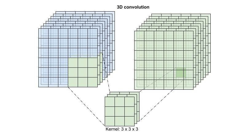
この演算は time * height * width * channels の入力を取って channels 出力を生成します（入力チャンネル数と出力チャンネル数が同じであることが前提です）。つまり、カーネルサイズが (3 x 3 x 3) の 3D 畳み込みレイヤーには、27 * channels ** 2 のエントリを持つ重み行列が必要となります。基準とする論文では、畳み込みを因数分解することがより効果的で効率的なアプローチという結果が導かれています。単一の 3D 畳み込みで時間次元と空間次元を処理するのではなく、空間と時間の次元を個別に処理する "(2+1)D" 畳み込みが提案されています。以下の図は、空間と時間で因数分解した (2 + 1)D 畳み込みを示しています。

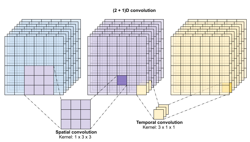
このアプローチの主なメリットは、パラメータ数が減ることにあります。(2 + 1)D 畳み込みでは、空間畳み込みは形状 (1, width, height) のデータを取るのに対し、時間畳み込みは形状 (time, 1, 1) のデータを取ります。たとえば、カーネルサイズが (3 x 3 x 3) の (2 + 1)D 畳み込みでは、サイズ (9 * channels**2) + (3 * channels**2) の重み行列が必要となり、これは、完全な 3D 畳み込みの半分です。このチュートリアルでは、ResNet の各畳み込みを (2+1)D 畳み込みが置き換わった (2 + 1)D ResNet18 を実装します。

# Define the dimensions of one frame in the set of frames created
HEIGHT = 224
WIDTH = 224

class Conv2Plus1D(keras.layers.Layer):
  def __init__(self, filters, kernel_size, padding):
    """
      A sequence of convolutional layers that first apply the convolution operation over the
      spatial dimensions, and then the temporal dimension. 
    """
    super().__init__()
    self.seq = keras.Sequential([  
        # Spatial decomposition
        layers.Conv3D(filters=filters,
                      kernel_size=(1, kernel_size[1], kernel_size[2]),
                      padding=padding),
        # Temporal decomposition
        layers.Conv3D(filters=filters, 
                      kernel_size=(kernel_size[0], 1, 1),
                      padding=padding)
        ])

  def call(self, x):
    return self.seq(x)

ResNet モデルは、一連の残差ブロックから作られています。残差ブロックには 2 つの分岐があります。メインの分岐は計算を実行しますが、勾配を流すのが困難です。残差分岐はメインの計算をバイパスして、ほぼ入力をメイン分岐の出力に追加するだけです。勾配は、この文器を容易に流れるため、損失関数からすべての残差ブロックのメイン分岐にたどり着く簡単な経路は存在することになります。これにより、勾配消失の問題が回避されます。

残差ブロックのメイン分岐を次のクラスで作成します。標準的な ResNet の構造とは対照に、これは layers.Conv2D ではなく Conv2Plus1D レイヤーを使用します。

class ResidualMain(keras.layers.Layer):
  """
    Residual block of the model with convolution, layer normalization, and the
    activation function, ReLU.
  """
  def __init__(self, filters, kernel_size):
    super().__init__()
    self.seq = keras.Sequential([
        Conv2Plus1D(filters=filters,
                    kernel_size=kernel_size,
                    padding='same'),
        layers.LayerNormalization(),
        layers.ReLU(),
        Conv2Plus1D(filters=filters, 
                    kernel_size=kernel_size,
                    padding='same'),
        layers.LayerNormalization()
    ])

  def call(self, x):
    return self.seq(x)

メイン分岐に残差分岐を追加するには、同じサイズである必要があります。以下の Project レイヤーは、チャンネルの数が分岐で変更されるケースに対処するものです。具体的には、一連の密結合レイヤーと正規化が追加されています。

class Project(keras.layers.Layer):
  """
    Project certain dimensions of the tensor as the data is passed through different 
    sized filters and downsampled. 
  """
  def __init__(self, units):
    super().__init__()
    self.seq = keras.Sequential([
        layers.Dense(units),
        layers.LayerNormalization()
    ])

  def call(self, x):
    return self.seq(x)

add_residual_block を使用して、モデルのレイヤー間にスキップ結合を導入します。

def add_residual_block(input, filters, kernel_size):
  """
    Add residual blocks to the model. If the last dimensions of the input data
    and filter size does not match, project it such that last dimension matches.
  """
  out = ResidualMain(filters, 
                     kernel_size)(input)

  res = input
  # Using the Keras functional APIs, project the last dimension of the tensor to
  # match the new filter size
  if out.shape[-1] != input.shape[-1]:
    res = Project(out.shape[-1])(res)

  return layers.add([res, out])

データのダウンサンプリングを行うには、動画サイズの変更が必要です。特に、動画フレームをダウンサンプリングすると、モデルがフレームの特定の箇所を調べてある行動に固有の可能性のあるパターンを検出することができます。重要でない情報は、ダウンサンプリングを通じて破棄することが可能です。さらに、動画のサイズを変更することで、次元を縮小できるため、モデルでの処理が高速化されます。

class ResizeVideo(keras.layers.Layer):
  def __init__(self, height, width):
    super().__init__()
    self.height = height
    self.width = width
    self.resizing_layer = layers.Resizing(self.height, self.width)

  def call(self, video):
    """
      Use the einops library to resize the tensor.  

      Args:
        video: Tensor representation of the video, in the form of a set of frames.

      Return:
        A downsampled size of the video according to the new height and width it should be resized to.
    """
    # b stands for batch size, t stands for time, h stands for height, 
    # w stands for width, and c stands for the number of channels.
    old_shape = einops.parse_shape(video, 'b t h w c')
    images = einops.rearrange(video, 'b t h w c -> (b t) h w c')
    images = self.resizing_layer(images)
    videos = einops.rearrange(
        images, '(b t) h w c -> b t h w c',
        t = old_shape['t'])
    return videos

Keras Functional API を使って、残差ネットワークを構築します。

input_shape = (None, 10, HEIGHT, WIDTH, 3)
input = layers.Input(shape=(input_shape[1:]))
x = input

x = Conv2Plus1D(filters=16, kernel_size=(3, 7, 7), padding='same')(x)
x = layers.BatchNormalization()(x)
x = layers.ReLU()(x)
x = ResizeVideo(HEIGHT // 2, WIDTH // 2)(x)

# Block 1
x = add_residual_block(x, 16, (3, 3, 3))
x = ResizeVideo(HEIGHT // 4, WIDTH // 4)(x)

# Block 2
x = add_residual_block(x, 32, (3, 3, 3))
x = ResizeVideo(HEIGHT // 8, WIDTH // 8)(x)

# Block 3
x = add_residual_block(x, 64, (3, 3, 3))
x = ResizeVideo(HEIGHT // 16, WIDTH // 16)(x)

# Block 4
x = add_residual_block(x, 128, (3, 3, 3))

x = layers.GlobalAveragePooling3D()(x)
x = layers.Flatten()(x)
x = layers.Dense(10)(x)

model = keras.Model(input, x)

frames, label = next(iter(train_ds))
model.build(frames)

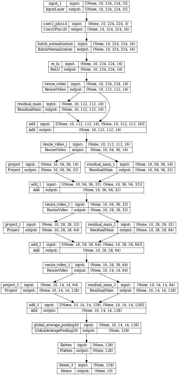
# Visualize the model
keras.utils.plot_model(model, expand_nested=True, dpi=60, show_shapes=True)

モデルのトレーニング

このチュートリアルでは、tf.keras.optimizers.Adam オプティマイザと tf.keras.losses.SparseCategoricalCrossentropy 損失関数を選択します。metrics 引数を使用して、各ステップでのモデルパフォーマンスの精度を確認します。

model.compile(loss = keras.losses.SparseCategoricalCrossentropy(from_logits=True), 
              optimizer = keras.optimizers.Adam(learning_rate = 0.0001), 
              metrics = ['accuracy'])

Keras Model.fit メソッドを使って、モデルを 50 エポック、トレーニングします。

注意: このサンプルモデルは、このチュートリアルに合理的な時間でトレーニングできるように、より少ないデータポイント（300 個のトレーニングサンプルと 100 個の検証サンプル）でトレーニングされています。また、このサンプルモデルのトレーニングには 1 時間以上かかる可能性があります。

history = model.fit(x = train_ds,
                    epochs = 50, 
                    validation_data = val_ds)

Epoch 1/50
WARNING: All log messages before absl::InitializeLog() is called are written to STDERR
I0000 00:00:1705001118.350866  129571 device_compiler.h:186] Compiled cluster using XLA!  This line is logged at most once for the lifetime of the process.
38/38 [==============================] - 81s 2s/step - loss: 2.6245 - accuracy: 0.1000 - val_loss: 2.5623 - val_accuracy: 0.1000
Epoch 2/50
38/38 [==============================] - 59s 2s/step - loss: 2.3280 - accuracy: 0.1567 - val_loss: 2.4639 - val_accuracy: 0.1000
Epoch 3/50
38/38 [==============================] - 59s 2s/step - loss: 2.2286 - accuracy: 0.1933 - val_loss: 2.1820 - val_accuracy: 0.2000
Epoch 4/50
38/38 [==============================] - 59s 2s/step - loss: 2.1448 - accuracy: 0.2600 - val_loss: 2.4221 - val_accuracy: 0.1600
Epoch 5/50
38/38 [==============================] - 59s 2s/step - loss: 2.0234 - accuracy: 0.2967 - val_loss: 2.4969 - val_accuracy: 0.2400
Epoch 6/50
38/38 [==============================] - 59s 2s/step - loss: 1.9068 - accuracy: 0.3333 - val_loss: 2.6993 - val_accuracy: 0.1500
Epoch 7/50
38/38 [==============================] - 59s 2s/step - loss: 1.9412 - accuracy: 0.2867 - val_loss: 2.3172 - val_accuracy: 0.2800
Epoch 8/50
38/38 [==============================] - 59s 2s/step - loss: 1.7902 - accuracy: 0.3400 - val_loss: 1.9949 - val_accuracy: 0.4000
Epoch 9/50
38/38 [==============================] - 59s 2s/step - loss: 1.7993 - accuracy: 0.3267 - val_loss: 2.6475 - val_accuracy: 0.2200
Epoch 10/50
38/38 [==============================] - 59s 2s/step - loss: 1.7501 - accuracy: 0.3500 - val_loss: 1.7358 - val_accuracy: 0.4700
Epoch 11/50
38/38 [==============================] - 59s 2s/step - loss: 1.6817 - accuracy: 0.3300 - val_loss: 2.1962 - val_accuracy: 0.2600
Epoch 12/50
38/38 [==============================] - 59s 2s/step - loss: 1.6873 - accuracy: 0.3400 - val_loss: 2.1749 - val_accuracy: 0.3100
Epoch 13/50
38/38 [==============================] - 59s 2s/step - loss: 1.5595 - accuracy: 0.4200 - val_loss: 1.9248 - val_accuracy: 0.3500
Epoch 14/50
38/38 [==============================] - 59s 2s/step - loss: 1.5023 - accuracy: 0.4233 - val_loss: 2.2648 - val_accuracy: 0.2300
Epoch 15/50
38/38 [==============================] - 59s 2s/step - loss: 1.4752 - accuracy: 0.4333 - val_loss: 1.6515 - val_accuracy: 0.4400
Epoch 16/50
38/38 [==============================] - 59s 2s/step - loss: 1.4280 - accuracy: 0.4833 - val_loss: 1.6030 - val_accuracy: 0.4200
Epoch 17/50
38/38 [==============================] - 59s 2s/step - loss: 1.3430 - accuracy: 0.5133 - val_loss: 1.6696 - val_accuracy: 0.3600
Epoch 18/50
38/38 [==============================] - 59s 2s/step - loss: 1.2448 - accuracy: 0.5467 - val_loss: 1.4545 - val_accuracy: 0.4800
Epoch 19/50
38/38 [==============================] - 59s 2s/step - loss: 1.3266 - accuracy: 0.5300 - val_loss: 1.3705 - val_accuracy: 0.4900
Epoch 20/50
38/38 [==============================] - 60s 2s/step - loss: 1.2845 - accuracy: 0.5600 - val_loss: 1.2928 - val_accuracy: 0.4700
Epoch 21/50
38/38 [==============================] - 59s 2s/step - loss: 1.1950 - accuracy: 0.5533 - val_loss: 1.4048 - val_accuracy: 0.4500
Epoch 22/50
38/38 [==============================] - 59s 2s/step - loss: 1.1403 - accuracy: 0.5600 - val_loss: 1.3348 - val_accuracy: 0.5100
Epoch 23/50
38/38 [==============================] - 59s 2s/step - loss: 1.0866 - accuracy: 0.6033 - val_loss: 1.2005 - val_accuracy: 0.5800
Epoch 24/50
38/38 [==============================] - 59s 2s/step - loss: 1.1717 - accuracy: 0.5433 - val_loss: 1.1050 - val_accuracy: 0.6100
Epoch 25/50
38/38 [==============================] - 59s 2s/step - loss: 1.0358 - accuracy: 0.6267 - val_loss: 1.3834 - val_accuracy: 0.5700
Epoch 26/50
38/38 [==============================] - 59s 2s/step - loss: 1.0719 - accuracy: 0.6033 - val_loss: 1.1959 - val_accuracy: 0.5600
Epoch 27/50
38/38 [==============================] - 59s 2s/step - loss: 0.9432 - accuracy: 0.6900 - val_loss: 1.0664 - val_accuracy: 0.6200
Epoch 28/50
38/38 [==============================] - 59s 2s/step - loss: 0.9006 - accuracy: 0.6767 - val_loss: 1.0215 - val_accuracy: 0.6300
Epoch 29/50
38/38 [==============================] - 59s 2s/step - loss: 0.8258 - accuracy: 0.7067 - val_loss: 1.0910 - val_accuracy: 0.6400
Epoch 30/50
38/38 [==============================] - 59s 2s/step - loss: 0.9075 - accuracy: 0.6633 - val_loss: 1.1556 - val_accuracy: 0.6100
Epoch 31/50
38/38 [==============================] - 60s 2s/step - loss: 0.8113 - accuracy: 0.7367 - val_loss: 1.0003 - val_accuracy: 0.6500
Epoch 32/50
38/38 [==============================] - 59s 2s/step - loss: 0.7484 - accuracy: 0.7667 - val_loss: 0.9289 - val_accuracy: 0.6800
Epoch 33/50
38/38 [==============================] - 59s 2s/step - loss: 0.8410 - accuracy: 0.7167 - val_loss: 0.9175 - val_accuracy: 0.6700
Epoch 34/50
38/38 [==============================] - 59s 2s/step - loss: 0.7001 - accuracy: 0.7800 - val_loss: 1.1768 - val_accuracy: 0.6000
Epoch 35/50
38/38 [==============================] - 59s 2s/step - loss: 0.7628 - accuracy: 0.7433 - val_loss: 1.0342 - val_accuracy: 0.5800
Epoch 36/50
38/38 [==============================] - 59s 2s/step - loss: 0.9521 - accuracy: 0.6467 - val_loss: 1.0204 - val_accuracy: 0.5900
Epoch 37/50
38/38 [==============================] - 59s 2s/step - loss: 0.7355 - accuracy: 0.7433 - val_loss: 1.0955 - val_accuracy: 0.6700
Epoch 38/50
38/38 [==============================] - 59s 2s/step - loss: 0.6927 - accuracy: 0.7333 - val_loss: 1.1643 - val_accuracy: 0.5600
Epoch 39/50
38/38 [==============================] - 59s 2s/step - loss: 0.8830 - accuracy: 0.6500 - val_loss: 1.0390 - val_accuracy: 0.5600
Epoch 40/50
38/38 [==============================] - 59s 2s/step - loss: 0.6603 - accuracy: 0.7700 - val_loss: 1.0357 - val_accuracy: 0.7000
Epoch 41/50
38/38 [==============================] - 59s 2s/step - loss: 0.6442 - accuracy: 0.7867 - val_loss: 1.0123 - val_accuracy: 0.6800
Epoch 42/50
38/38 [==============================] - 59s 2s/step - loss: 0.7143 - accuracy: 0.7233 - val_loss: 0.9508 - val_accuracy: 0.6800
Epoch 43/50
38/38 [==============================] - 59s 2s/step - loss: 0.6025 - accuracy: 0.8133 - val_loss: 1.2498 - val_accuracy: 0.5700
Epoch 44/50
38/38 [==============================] - 59s 2s/step - loss: 0.6129 - accuracy: 0.7767 - val_loss: 0.9852 - val_accuracy: 0.6000
Epoch 45/50
38/38 [==============================] - 59s 2s/step - loss: 0.6118 - accuracy: 0.7900 - val_loss: 0.9424 - val_accuracy: 0.6400
Epoch 46/50
38/38 [==============================] - 60s 2s/step - loss: 0.5690 - accuracy: 0.8033 - val_loss: 0.9257 - val_accuracy: 0.6800
Epoch 47/50
38/38 [==============================] - 59s 2s/step - loss: 0.5964 - accuracy: 0.8033 - val_loss: 1.1536 - val_accuracy: 0.6200
Epoch 48/50
38/38 [==============================] - 59s 2s/step - loss: 0.5571 - accuracy: 0.7967 - val_loss: 0.7774 - val_accuracy: 0.7100
Epoch 49/50
38/38 [==============================] - 59s 2s/step - loss: 0.5236 - accuracy: 0.8467 - val_loss: 0.9425 - val_accuracy: 0.6900
Epoch 50/50
38/38 [==============================] - 59s 2s/step - loss: 0.4978 - accuracy: 0.8267 - val_loss: 0.7630 - val_accuracy: 0.7300

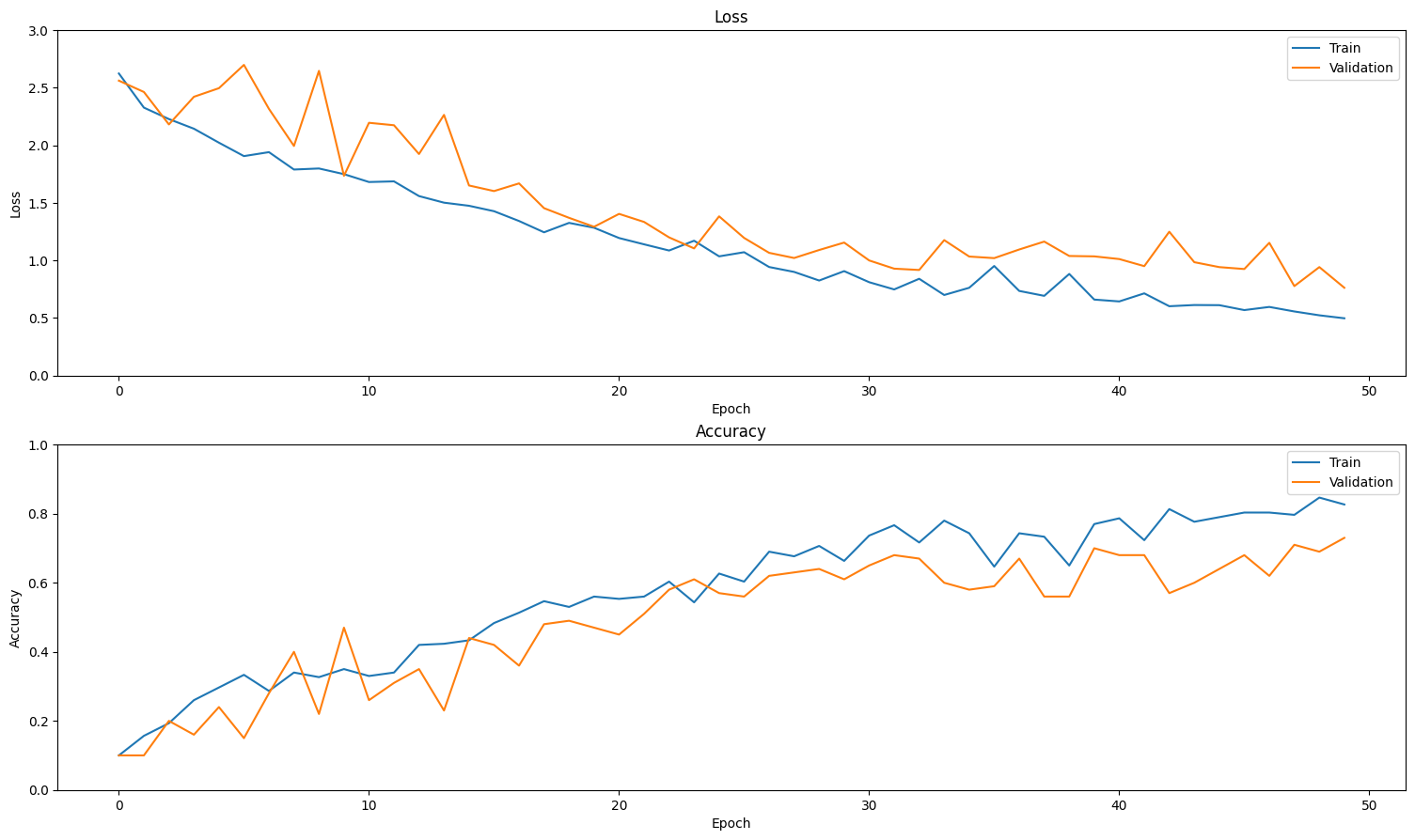
結果を可視化する

トレーニングセットと検証セットで損失と精度のプロットを作成します。

def plot_history(history):
  """
    Plotting training and validation learning curves.

    Args:
      history: model history with all the metric measures
  """
  fig, (ax1, ax2) = plt.subplots(2)

  fig.set_size_inches(18.5, 10.5)

  # Plot loss
  ax1.set_title('Loss')
  ax1.plot(history.history['loss'], label = 'train')
  ax1.plot(history.history['val_loss'], label = 'test')
  ax1.set_ylabel('Loss')

  # Determine upper bound of y-axis
  max_loss = max(history.history['loss'] + history.history['val_loss'])

  ax1.set_ylim([0, np.ceil(max_loss)])
  ax1.set_xlabel('Epoch')
  ax1.legend(['Train', 'Validation']) 

  # Plot accuracy
  ax2.set_title('Accuracy')
  ax2.plot(history.history['accuracy'],  label = 'train')
  ax2.plot(history.history['val_accuracy'], label = 'test')
  ax2.set_ylabel('Accuracy')
  ax2.set_ylim([0, 1])
  ax2.set_xlabel('Epoch')
  ax2.legend(['Train', 'Validation'])

  plt.show()

plot_history(history)

モデルを評価する

Keras Model.evaluate を使用して、テストデータセットで損失と精度を取得します。

注意: このチュートリアルのサンプルモデルは、合理的な時間でトレーニングできるように、UCF101 データセットのサブセットを使用しています。ハイパーパラメータのチューニングをさらに行ったり、トレーニングデータを増やすことで、精度と損失を改善できる可能性があります。

model.evaluate(test_ds, return_dict=True)

13/13 [==============================] - 12s 893ms/step - loss: 0.6833 - accuracy: 0.7700
{'loss': 0.6833138465881348, 'accuracy': 0.7699999809265137}

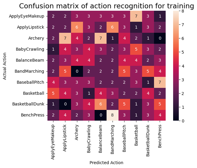
モデルパフォーマンスをさらに可視化するには、混同行列を使用します。混同行列では、精度を超えて分類モデルのパフォーマンスを評価することができます。このマルチクラス分類問題の混同行列を作成するために、テストセットの実際の値と予測される値を取得します。

def get_actual_predicted_labels(dataset): 
  """
    Create a list of actual ground truth values and the predictions from the model.

    Args:
      dataset: An iterable data structure, such as a TensorFlow Dataset, with features and labels.

    Return:
      Ground truth and predicted values for a particular dataset.
  """
  actual = [labels for _, labels in dataset.unbatch()]
  predicted = model.predict(dataset)

  actual = tf.stack(actual, axis=0)
  predicted = tf.concat(predicted, axis=0)
  predicted = tf.argmax(predicted, axis=1)

  return actual, predicted

def plot_confusion_matrix(actual, predicted, labels, ds_type):
  cm = tf.math.confusion_matrix(actual, predicted)
  ax = sns.heatmap(cm, annot=True, fmt='g')
  sns.set(rc={'figure.figsize':(12, 12)})
  sns.set(font_scale=1.4)
  ax.set_title('Confusion matrix of action recognition for ' + ds_type)
  ax.set_xlabel('Predicted Action')
  ax.set_ylabel('Actual Action')
  plt.xticks(rotation=90)
  plt.yticks(rotation=0)
  ax.xaxis.set_ticklabels(labels)
  ax.yaxis.set_ticklabels(labels)

fg = FrameGenerator(subset_paths['train'], n_frames, training=True)
labels = list(fg.class_ids_for_name.keys())

actual, predicted = get_actual_predicted_labels(train_ds)
plot_confusion_matrix(actual, predicted, labels, 'training')

38/38 [==============================] - 37s 936ms/step

actual, predicted = get_actual_predicted_labels(test_ds)
plot_confusion_matrix(actual, predicted, labels, 'test')

13/13 [==============================] - 12s 891ms/step

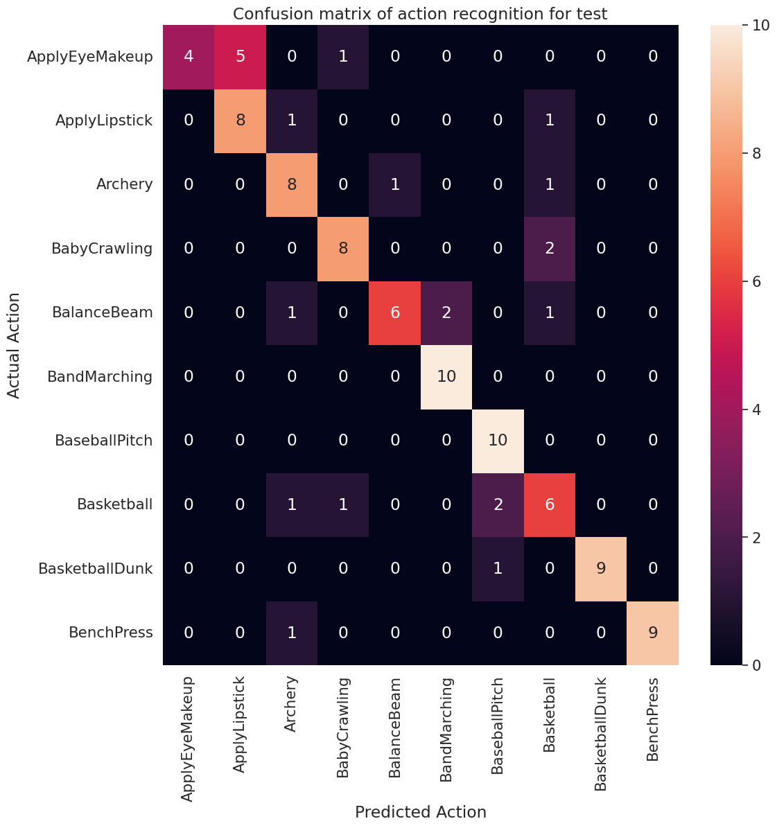
各クラスの適合率と再現率の値は、混同行列を使用して計算することもできます。

def calculate_classification_metrics(y_actual, y_pred, labels):
  """
    Calculate the precision and recall of a classification model using the ground truth and
    predicted values. 

    Args:
      y_actual: Ground truth labels.
      y_pred: Predicted labels.
      labels: List of classification labels.

    Return:
      Precision and recall measures.
  """
  cm = tf.math.confusion_matrix(y_actual, y_pred)
  tp = np.diag(cm) # Diagonal represents true positives
  precision = dict()
  recall = dict()
  for i in range(len(labels)):
    col = cm[:, i]
    fp = np.sum(col) - tp[i] # Sum of column minus true positive is false negative

    row = cm[i, :]
    fn = np.sum(row) - tp[i] # Sum of row minus true positive, is false negative

    precision[labels[i]] = tp[i] / (tp[i] + fp) # Precision 

    recall[labels[i]] = tp[i] / (tp[i] + fn) # Recall

  return precision, recall

precision, recall = calculate_classification_metrics(actual, predicted, labels) # Test dataset

precision

{'ApplyEyeMakeup': 1.0,
 'ApplyLipstick': 0.6153846153846154,
 'Archery': 0.6666666666666666,
 'BabyCrawling': 0.8,
 'BalanceBeam': 0.8571428571428571,
 'BandMarching': 0.8333333333333334,
 'BaseballPitch': 0.7692307692307693,
 'Basketball': 0.5454545454545454,
 'BasketballDunk': 1.0,
 'BenchPress': 1.0}

recall

{'ApplyEyeMakeup': 0.4,
 'ApplyLipstick': 0.8,
 'Archery': 0.8,
 'BabyCrawling': 0.8,
 'BalanceBeam': 0.6,
 'BandMarching': 1.0,
 'BaseballPitch': 1.0,
 'Basketball': 0.6,
 'BasketballDunk': 0.9,
 'BenchPress': 0.9}

次のステップ

TensorFlow での動画の操作についての詳細は、以下のチュートリアルをご覧ください。

• 動画データを読み込む
• MoviNet でストリーミングの行動認識を実行する
• MoviNet を使った動画分類の転移学習