
| | |  Kaynağı GitHub'da görüntüleyin Kaynağı GitHub'da görüntüleyin |
Bu öğretici , bir Transformer modelini Portekizce'den İngilizce'ye veri kümesini çevirmek için eğitir . Bu, metin oluşturma ve dikkat bilgisini varsayan gelişmiş bir örnektir.
Transformer modelinin arkasındaki temel fikir, öz- dikkattir - bu dizinin bir temsilini hesaplamak için giriş dizisinin farklı konumlarına katılma yeteneği. Transformer, kendine dikkat eden katman yığınları oluşturur ve aşağıda Ölçekli nokta ürün dikkati ve Çok başlı dikkat bölümlerinde açıklanmıştır.
Bir transformatör modeli, RNN'ler veya CNN'ler yerine kendi kendine dikkat eden katman yığınlarını kullanarak değişken boyutlu girdileri işler. Bu genel mimarinin bir takım avantajları vardır:
- Veriler arasındaki zamansal/mekansal ilişkiler hakkında hiçbir varsayımda bulunmaz. Bu, bir dizi nesneyi işlemek için idealdir (örneğin, StarCraft birimleri ).
- Katman çıktıları, RNN gibi bir seri yerine paralel olarak hesaplanabilir.
- Uzaktaki öğeler, birçok RNN adımından veya evrişim katmanlarından geçmeden birbirlerinin çıktısını etkileyebilir (örneğin bkz. Scene Memory Transformer ).
- Uzun menzilli bağımlılıkları öğrenebilir. Bu, birçok sıralı görevde bir meydan okumadır.
Bu mimarinin dezavantajları şunlardır:
- Bir zaman serisi için, bir zaman adımının çıktısı, yalnızca girdiler ve mevcut gizli durum yerine tüm geçmiş üzerinden hesaplanır. Bu daha az verimli olabilir .
- Girdinin metin gibi zamansal/mekansal bir ilişkisi varsa, bazı konumsal kodlamalar eklenmelidir, aksi takdirde model etkili bir şekilde bir sözcük torbası görür.
Modeli bu defterde eğittikten sonra, Portekizce bir cümle girebilecek ve İngilizce çevirisini geri gönderebileceksiniz.
Kurmak
pip install tensorflow_datasetspip install -U tensorflow-text
import collections
import logging
import os
import pathlib
import re
import string
import sys
import time

import numpy as np
import matplotlib.pyplot as plt

import tensorflow_datasets as tfds
import tensorflow_text as text
import tensorflow as tf
logging.getLogger('tensorflow').setLevel(logging.ERROR) # suppress warnings
Veri Kümesini İndirin
TED Talks Açık Çeviri Projesi'nden Portekizce-İngilizce çeviri veri kümesini yüklemek için TensorFlow veri kümelerini kullanın.
Bu veri seti yaklaşık 50000 eğitim örneği, 1100 doğrulama örneği ve 2000 test örneği içermektedir.
examples, metadata = tfds.load('ted_hrlr_translate/pt_to_en', with_info=True,
                               as_supervised=True)
train_examples, val_examples = examples['train'], examples['validation']
TensorFlow veri kümeleri tarafından döndürülen tf.data.Dataset nesnesi, metin örnekleri çiftleri verir:
for pt_examples, en_examples in train_examples.batch(3).take(1):
  for pt in pt_examples.numpy():
    print(pt.decode('utf-8'))

  print()

  for en in en_examples.numpy():
    print(en.decode('utf-8'))
e quando melhoramos a procura , tiramos a única vantagem da impressão , que é a serendipidade .
mas e se estes fatores fossem ativos ?
mas eles não tinham a curiosidade de me testar .

and when you improve searchability , you actually take away the one advantage of print , which is serendipity .
but what if it were active ?
but they did n't test for curiosity .
Metin tokenizasyonu ve detokenization
Bir modeli doğrudan metin üzerinde eğitemezsiniz. Metnin önce bazı sayısal temsillere dönüştürülmesi gerekir. Tipik olarak, metni, bir gömmede dizinler olarak kullanılan belirteç kimlikleri dizilerine dönüştürürsünüz.
Subword tokenizer öğreticisinde popüler bir uygulama gösterilmektedir , bu veri kümesi için optimize edilmiş alt kelime belirteçleri ( text.BertTokenizer ) oluşturur ve bunları bir save_model içinde dışa aktarır .
saved_model indirin ve açın ve içe aktarın:
model_name = "ted_hrlr_translate_pt_en_converter"
tf.keras.utils.get_file(
    f"{model_name}.zip",
    f"https://storage.googleapis.com/download.tensorflow.org/models/{model_name}.zip",
    cache_dir='.', cache_subdir='', extract=True
)
Downloading data from https://storage.googleapis.com/download.tensorflow.org/models/ted_hrlr_translate_pt_en_converter.zip
188416/184801 [==============================] - 0s 0us/step
196608/184801 [===============================] - 0s 0us/step
'./ted_hrlr_translate_pt_en_converter.zip'
-yer tutucu12 l10n-yer
tokenizers = tf.saved_model.load(model_name)
tf.saved_model , biri İngilizce, diğeri Portekizce için olmak üzere iki metin belirteci içerir. Her ikisi de aynı yöntemlere sahiptir:
[item for item in dir(tokenizers.en) if not item.startswith('_')]
['detokenize',
 'get_reserved_tokens',
 'get_vocab_path',
 'get_vocab_size',
 'lookup',
 'tokenize',
 'tokenizer',
 'vocab']
tokenize yöntemi, bir dizi diziyi dolgulu bir simge kimliği grubuna dönüştürür. Bu yöntem noktalama işaretlerini, küçük harfleri böler ve simgeleştirmeden önce girişi unicode olarak normalleştirir. Girdi verileri zaten standartlaştırıldığı için bu standardizasyon burada görünmez.
for en in en_examples.numpy():
  print(en.decode('utf-8'))
and when you improve searchability , you actually take away the one advantage of print , which is serendipity .
but what if it were active ?
but they did n't test for curiosity .
yer tutucu17 l10n-yer
encoded = tokenizers.en.tokenize(en_examples)

for row in encoded.to_list():
  print(row)
[2, 72, 117, 79, 1259, 1491, 2362, 13, 79, 150, 184, 311, 71, 103, 2308, 74, 2679, 13, 148, 80, 55, 4840, 1434, 2423, 540, 15, 3]
[2, 87, 90, 107, 76, 129, 1852, 30, 3]
[2, 87, 83, 149, 50, 9, 56, 664, 85, 2512, 15, 3]
detokenize yöntemi, bu belirteç kimliklerini insan tarafından okunabilir metne dönüştürmeye çalışır:
round_trip = tokenizers.en.detokenize(encoded)
for line in round_trip.numpy():
  print(line.decode('utf-8'))
and when you improve searchability , you actually take away the one advantage of print , which is serendipity .
but what if it were active ?
but they did n ' t test for curiosity .
Alt düzey lookup yöntemi, belirteç kimliklerini belirteç metnine dönüştürür:
tokens = tokenizers.en.lookup(encoded)
tokens
<tf.RaggedTensor [[b'[START]', b'and', b'when', b'you', b'improve', b'search', b'##ability',
  b',', b'you', b'actually', b'take', b'away', b'the', b'one', b'advantage',
  b'of', b'print', b',', b'which', b'is', b's', b'##ere', b'##nd', b'##ip',
  b'##ity', b'.', b'[END]']                                                 ,
 [b'[START]', b'but', b'what', b'if', b'it', b'were', b'active', b'?',
  b'[END]']                                                           ,
 [b'[START]', b'but', b'they', b'did', b'n', b"'", b't', b'test', b'for',
  b'curiosity', b'.', b'[END]']                                          ]>
Burada belirteçlerin "alt kelime" yönünü görebilirsiniz. "Aranabilirlik" kelimesi "arama ##yetenek" ve "şans" kelimesi "s ##ere ##nd ##ip ##ity" olarak ayrıştırılır
Giriş ardışık düzenini ayarla
Eğitime uygun bir girdi ardışık düzeni oluşturmak için veri kümesine bazı dönüşümler uygulayacaksınız.
Bu işlev, ham metin gruplarını kodlamak için kullanılacaktır:
def tokenize_pairs(pt, en):
    pt = tokenizers.pt.tokenize(pt)
    # Convert from ragged to dense, padding with zeros.
    pt = pt.to_tensor()

    en = tokenizers.en.tokenize(en)
    # Convert from ragged to dense, padding with zeros.
    en = en.to_tensor()
    return pt, en
İşte verileri işleyen, karıştıran ve gruplandıran basit bir girdi ardışık düzeni:
BUFFER_SIZE = 20000
BATCH_SIZE = 64
def make_batches(ds):
  return (
      ds
      .cache()
      .shuffle(BUFFER_SIZE)
      .batch(BATCH_SIZE)
      .map(tokenize_pairs, num_parallel_calls=tf.data.AUTOTUNE)
      .prefetch(tf.data.AUTOTUNE))


train_batches = make_batches(train_examples)
val_batches = make_batches(val_examples)
konumsal kodlama
Dikkat katmanları, girdilerini sıralı bir sıra olmaksızın bir dizi vektör olarak görür. Bu model ayrıca tekrarlayan veya evrişimli katmanlar içermez. Bu nedenle, modele belirteçlerin cümle içindeki göreli konumu hakkında bazı bilgiler vermek için bir "konumsal kodlama" eklenir.
Konumsal kodlama vektörü, gömme vektörüne eklenir. Gömmeler, benzer anlama sahip belirteçlerin birbirine daha yakın olacağı d-boyutlu bir uzayda bir belirteci temsil eder. Ancak yerleştirmeler, bir cümledeki belirteçlerin göreli konumunu kodlamaz. Böylece konumsal kodlamayı ekledikten sonra, belirteçler anlamlarının benzerliğine ve d-boyutlu uzaydaki cümle içindeki konumlarına göre birbirine daha yakın olacaktır.
Konumsal kodlamayı hesaplama formülü aşağıdaki gibidir:
\[\Large{PE_{(pos, 2i)} = \sin(pos / 10000^{2i / d_{model} })} \]
\[\Large{PE_{(pos, 2i+1)} = \cos(pos / 10000^{2i / d_{model} })} \]
def get_angles(pos, i, d_model):
  angle_rates = 1 / np.power(10000, (2 * (i//2)) / np.float32(d_model))
  return pos * angle_rates
def positional_encoding(position, d_model):
  angle_rads = get_angles(np.arange(position)[:, np.newaxis],
                          np.arange(d_model)[np.newaxis, :],
                          d_model)

  # apply sin to even indices in the array; 2i
  angle_rads[:, 0::2] = np.sin(angle_rads[:, 0::2])

  # apply cos to odd indices in the array; 2i+1
  angle_rads[:, 1::2] = np.cos(angle_rads[:, 1::2])

  pos_encoding = angle_rads[np.newaxis, ...]

  return tf.cast(pos_encoding, dtype=tf.float32)
n, d = 2048, 512
pos_encoding = positional_encoding(n, d)
print(pos_encoding.shape)
pos_encoding = pos_encoding[0]

# Juggle the dimensions for the plot
pos_encoding = tf.reshape(pos_encoding, (n, d//2, 2))
pos_encoding = tf.transpose(pos_encoding, (2, 1, 0))
pos_encoding = tf.reshape(pos_encoding, (d, n))

plt.pcolormesh(pos_encoding, cmap='RdBu')
plt.ylabel('Depth')
plt.xlabel('Position')
plt.colorbar()
plt.show()
(1, 2048, 512)

maskeleme
Dizideki tüm pad belirteçlerini maskeleyin. Modelin dolguyu girdi olarak görmemesini sağlar. Maske, ped değeri 0 nerede olduğunu gösterir: bu konumlarda 1 , aksi takdirde 0 verir.
def create_padding_mask(seq):
  seq = tf.cast(tf.math.equal(seq, 0), tf.float32)

  # add extra dimensions to add the padding
  # to the attention logits.
  return seq[:, tf.newaxis, tf.newaxis, :]  # (batch_size, 1, 1, seq_len)
x = tf.constant([[7, 6, 0, 0, 1], [1, 2, 3, 0, 0], [0, 0, 0, 4, 5]])
create_padding_mask(x)
<tf.Tensor: shape=(3, 1, 1, 5), dtype=float32, numpy=
array([[[[0., 0., 1., 1., 0.]]],


       [[[0., 0., 0., 1., 1.]]],


       [[[1., 1., 1., 0., 0.]]]], dtype=float32)>
İleriye dönük maske, bir sıradaki gelecek belirteçleri maskelemek için kullanılır. Başka bir deyişle, maske hangi girdilerin kullanılmaması gerektiğini belirtir.
Bu, üçüncü jetonu tahmin etmek için yalnızca birinci ve ikinci jetonun kullanılacağı anlamına gelir. Dördüncü belirteci tahmin etmek için benzer şekilde, yalnızca birinci, ikinci ve üçüncü belirteçler kullanılacaktır.
def create_look_ahead_mask(size):
  mask = 1 - tf.linalg.band_part(tf.ones((size, size)), -1, 0)
  return mask  # (seq_len, seq_len)
x = tf.random.uniform((1, 3))
temp = create_look_ahead_mask(x.shape[1])
temp
<tf.Tensor: shape=(3, 3), dtype=float32, numpy=
array([[0., 1., 1.],
       [0., 0., 1.],
       [0., 0., 0.]], dtype=float32)>
Ölçekli nokta ürün dikkati
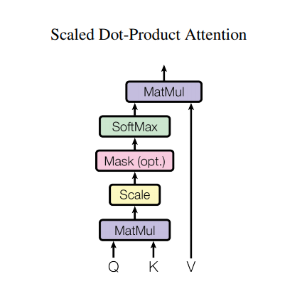
Transformatör tarafından kullanılan dikkat fonksiyonu üç giriş alır: Q (sorgu), K (anahtar), V (değer). Dikkat ağırlıklarını hesaplamak için kullanılan denklem:
\[\Large{Attention(Q, K, V) = softmax_k\left(\frac{QK^T}{\sqrt{d_k} }\right) V} \]
Nokta-ürün dikkati, derinliğin karekökü faktörüyle ölçeklenir. Bu, büyük derinlik değerleri için, nokta çarpım, çok sert bir softmax ile sonuçlanan küçük gradyanlara sahip olduğu yerlerde softmax işlevini iterek büyüklük olarak büyüdüğü için yapılır.
Örneğin, Q ve K ortalamasının 0 ve varyansının 1 olduğunu düşünün. Bunların matris çarpımlarının ortalaması 0 ve varyansı dk olacaktır. Bu nedenle, ölçekleme için dk karekökü kullanılır, böylece dk değerinden bağımsız olarak tutarlı bir varyans elde edersiniz. Varyans çok düşükse, çıktı etkin bir şekilde optimize edemeyecek kadar düz olabilir. Varyans çok yüksekse, softmax başlangıçta doygun hale gelebilir ve öğrenmeyi zorlaştırabilir.
Maske -1e9 ile çarpılır (negatif sonsuza yakın). Bu yapılır çünkü maske, Q ve K'nin ölçeklenmiş matris çarpımı ile toplanır ve bir softmax'tan hemen önce uygulanır. Amaç, bu hücreleri sıfırlamaktır ve softmax'a yönelik büyük negatif girdiler, çıktıda sıfıra yakındır.
def scaled_dot_product_attention(q, k, v, mask):
  """Calculate the attention weights.
  q, k, v must have matching leading dimensions.
  k, v must have matching penultimate dimension, i.e.: seq_len_k = seq_len_v.
  The mask has different shapes depending on its type(padding or look ahead)
  but it must be broadcastable for addition.

  Args:
    q: query shape == (..., seq_len_q, depth)
    k: key shape == (..., seq_len_k, depth)
    v: value shape == (..., seq_len_v, depth_v)
    mask: Float tensor with shape broadcastable
          to (..., seq_len_q, seq_len_k). Defaults to None.

  Returns:
    output, attention_weights
  """

  matmul_qk = tf.matmul(q, k, transpose_b=True)  # (..., seq_len_q, seq_len_k)

  # scale matmul_qk
  dk = tf.cast(tf.shape(k)[-1], tf.float32)
  scaled_attention_logits = matmul_qk / tf.math.sqrt(dk)

  # add the mask to the scaled tensor.
  if mask is not None:
    scaled_attention_logits += (mask * -1e9)

  # softmax is normalized on the last axis (seq_len_k) so that the scores
  # add up to 1.
  attention_weights = tf.nn.softmax(scaled_attention_logits, axis=-1)  # (..., seq_len_q, seq_len_k)

  output = tf.matmul(attention_weights, v)  # (..., seq_len_q, depth_v)

  return output, attention_weights
Softmax normalizasyonu K üzerinde yapıldığından, değerleri Q'ya verilen önem miktarını belirler.
Çıktı, dikkat ağırlıklarının ve V (değer) vektörünün çarpımını temsil eder. Bu, odaklanmak istediğiniz belirteçlerin olduğu gibi tutulmasını ve alakasız belirteçlerin temizlenmesini sağlar.
def print_out(q, k, v):
  temp_out, temp_attn = scaled_dot_product_attention(
      q, k, v, None)
  print('Attention weights are:')
  print(temp_attn)
  print('Output is:')
  print(temp_out)
np.set_printoptions(suppress=True)

temp_k = tf.constant([[10, 0, 0],
                      [0, 10, 0],
                      [0, 0, 10],
                      [0, 0, 10]], dtype=tf.float32)  # (4, 3)

temp_v = tf.constant([[1, 0],
                      [10, 0],
                      [100, 5],
                      [1000, 6]], dtype=tf.float32)  # (4, 2)

# This `query` aligns with the second `key`,
# so the second `value` is returned.
temp_q = tf.constant([[0, 10, 0]], dtype=tf.float32)  # (1, 3)
print_out(temp_q, temp_k, temp_v)
Attention weights are:
tf.Tensor([[0. 1. 0. 0.]], shape=(1, 4), dtype=float32)
Output is:
tf.Tensor([[10.  0.]], shape=(1, 2), dtype=float32)
# This query aligns with a repeated key (third and fourth),
# so all associated values get averaged.
temp_q = tf.constant([[0, 0, 10]], dtype=tf.float32)  # (1, 3)
print_out(temp_q, temp_k, temp_v)
Attention weights are:
tf.Tensor([[0.  0.  0.5 0.5]], shape=(1, 4), dtype=float32)
Output is:
tf.Tensor([[550.    5.5]], shape=(1, 2), dtype=float32)
# This query aligns equally with the first and second key,
# so their values get averaged.
temp_q = tf.constant([[10, 10, 0]], dtype=tf.float32)  # (1, 3)
print_out(temp_q, temp_k, temp_v)
Attention weights are:
tf.Tensor([[0.5 0.5 0.  0. ]], shape=(1, 4), dtype=float32)
Output is:
tf.Tensor([[5.5 0. ]], shape=(1, 2), dtype=float32)
Tüm sorguları birlikte iletin.
temp_q = tf.constant([[0, 0, 10],
                      [0, 10, 0],
                      [10, 10, 0]], dtype=tf.float32)  # (3, 3)
print_out(temp_q, temp_k, temp_v)
Attention weights are:
tf.Tensor(
[[0.  0.  0.5 0.5]
 [0.  1.  0.  0. ]
 [0.5 0.5 0.  0. ]], shape=(3, 4), dtype=float32)
Output is:
tf.Tensor(
[[550.    5.5]
 [ 10.    0. ]
 [  5.5   0. ]], shape=(3, 2), dtype=float32)
Çok kafalı dikkat
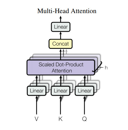
Çok kafalı dikkat dört bölümden oluşur:
- Doğrusal katmanlar.
- Ölçekli nokta-ürün dikkati.
- Son doğrusal katman.
Her çok başlı dikkat bloğu üç girdi alır; Q (sorgu), K (anahtar), V (değer). Bunlar, çok başlı dikkat işlevinden önce doğrusal (Yoğun) katmanlardan geçirilir.
Yukarıdaki şemada (K,Q,V) her bir dikkat kafası için ayrı lineer ( Dense ) katmanlardan geçirilmektedir. Basitlik/verimlilik için, aşağıdaki kod bunu, çıktı sayısı kadar çok sayıda num_heads ile tek bir yoğun katman kullanarak uygular. Çıktı, dikkat işlevi uygulanmadan önce (batch, num_heads, ...) şeklinde yeniden düzenlenir.
Yukarıda tanımlanan scaled_dot_product_attention işlevi, verimlilik için yayınlanan tek bir çağrıda uygulanır. Dikkat aşamasında uygun bir maske kullanılmalıdır. Her kafa için dikkat çıktısı daha sonra birleştirilir ( tf.transpose ve tf.reshape kullanılarak) ve son bir Dense katmandan geçirilir.
Tek bir dikkat başlığı yerine, Q, K ve V çoklu kafalara bölünür, çünkü modelin farklı konumlardaki farklı temsil altuzaylarından gelen bilgilere ortaklaşa katılmasını sağlar. Bölünmeden sonra her bir kafa azaltılmış bir boyuta sahiptir, bu nedenle toplam hesaplama maliyeti, tam boyutlu tek bir kafa dikkatiyle aynıdır.
class MultiHeadAttention(tf.keras.layers.Layer):
  def __init__(self, d_model, num_heads):
    super(MultiHeadAttention, self).__init__()
    self.num_heads = num_heads
    self.d_model = d_model

    assert d_model % self.num_heads == 0

    self.depth = d_model // self.num_heads

    self.wq = tf.keras.layers.Dense(d_model)
    self.wk = tf.keras.layers.Dense(d_model)
    self.wv = tf.keras.layers.Dense(d_model)

    self.dense = tf.keras.layers.Dense(d_model)

  def split_heads(self, x, batch_size):
    """Split the last dimension into (num_heads, depth).
    Transpose the result such that the shape is (batch_size, num_heads, seq_len, depth)
    """
    x = tf.reshape(x, (batch_size, -1, self.num_heads, self.depth))
    return tf.transpose(x, perm=[0, 2, 1, 3])

  def call(self, v, k, q, mask):
    batch_size = tf.shape(q)[0]

    q = self.wq(q)  # (batch_size, seq_len, d_model)
    k = self.wk(k)  # (batch_size, seq_len, d_model)
    v = self.wv(v)  # (batch_size, seq_len, d_model)

    q = self.split_heads(q, batch_size)  # (batch_size, num_heads, seq_len_q, depth)
    k = self.split_heads(k, batch_size)  # (batch_size, num_heads, seq_len_k, depth)
    v = self.split_heads(v, batch_size)  # (batch_size, num_heads, seq_len_v, depth)

    # scaled_attention.shape == (batch_size, num_heads, seq_len_q, depth)
    # attention_weights.shape == (batch_size, num_heads, seq_len_q, seq_len_k)
    scaled_attention, attention_weights = scaled_dot_product_attention(
        q, k, v, mask)

    scaled_attention = tf.transpose(scaled_attention, perm=[0, 2, 1, 3])  # (batch_size, seq_len_q, num_heads, depth)

    concat_attention = tf.reshape(scaled_attention,
                                  (batch_size, -1, self.d_model))  # (batch_size, seq_len_q, d_model)

    output = self.dense(concat_attention)  # (batch_size, seq_len_q, d_model)

    return output, attention_weights
Denemek için bir MultiHeadAttention katmanı oluşturun. Dizideki her konumda, y , MultiHeadAttention diğer tüm konumlarda 8 dikkat başlığının tümünü çalıştırır ve her konumda aynı uzunlukta yeni bir vektör döndürür.
temp_mha = MultiHeadAttention(d_model=512, num_heads=8)
y = tf.random.uniform((1, 60, 512))  # (batch_size, encoder_sequence, d_model)
out, attn = temp_mha(y, k=y, q=y, mask=None)
out.shape, attn.shape
(TensorShape([1, 60, 512]), TensorShape([1, 8, 60, 60]))
Nokta bilge ileri besleme ağı
Nokta bilge ileri beslemeli ağ, aralarında bir ReLU aktivasyonu bulunan tam bağlantılı iki katmandan oluşur.
def point_wise_feed_forward_network(d_model, dff):
  return tf.keras.Sequential([
      tf.keras.layers.Dense(dff, activation='relu'),  # (batch_size, seq_len, dff)
      tf.keras.layers.Dense(d_model)  # (batch_size, seq_len, d_model)
  ])
sample_ffn = point_wise_feed_forward_network(512, 2048)
sample_ffn(tf.random.uniform((64, 50, 512))).shape
TensorShape([64, 50, 512])
Kodlayıcı ve kod çözücü
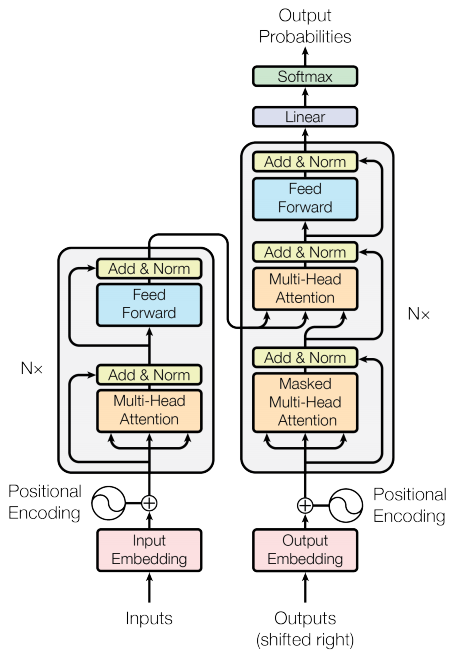
Transformatör modeli , dikkat modeliyle sıralamak için standart bir diziyle aynı genel modeli takip eder.
- Giriş cümlesi, dizideki her belirteç için bir çıktı üreten
Nkodlayıcı katmanından geçirilir. - Kod çözücü, bir sonraki kelimeyi tahmin etmek için kodlayıcının çıktısına ve kendi girdisine (öz-dikkat) katılır.
kodlayıcı katmanı
Her kodlayıcı katmanı, alt katmanlardan oluşur:
- Çok kafalı dikkat (dolgu maskesi ile)
- Nokta bilge ileri beslemeli ağlar.
Bu alt katmanların her birinin çevresinde artık bir bağlantı ve ardından bir katman normalizasyonu vardır. Artık bağlantılar, derin ağlarda kaybolan gradyan probleminden kaçınmaya yardımcı olur.
Her alt katmanın çıktısı LayerNorm(x + Sublayer(x)) . Normalleştirme, d_model (son) ekseninde yapılır. Transformatörde N adet kodlayıcı katmanı bulunmaktadır.
class EncoderLayer(tf.keras.layers.Layer):
  def __init__(self, d_model, num_heads, dff, rate=0.1):
    super(EncoderLayer, self).__init__()

    self.mha = MultiHeadAttention(d_model, num_heads)
    self.ffn = point_wise_feed_forward_network(d_model, dff)

    self.layernorm1 = tf.keras.layers.LayerNormalization(epsilon=1e-6)
    self.layernorm2 = tf.keras.layers.LayerNormalization(epsilon=1e-6)

    self.dropout1 = tf.keras.layers.Dropout(rate)
    self.dropout2 = tf.keras.layers.Dropout(rate)

  def call(self, x, training, mask):

    attn_output, _ = self.mha(x, x, x, mask)  # (batch_size, input_seq_len, d_model)
    attn_output = self.dropout1(attn_output, training=training)
    out1 = self.layernorm1(x + attn_output)  # (batch_size, input_seq_len, d_model)

    ffn_output = self.ffn(out1)  # (batch_size, input_seq_len, d_model)
    ffn_output = self.dropout2(ffn_output, training=training)
    out2 = self.layernorm2(out1 + ffn_output)  # (batch_size, input_seq_len, d_model)

    return out2
sample_encoder_layer = EncoderLayer(512, 8, 2048)

sample_encoder_layer_output = sample_encoder_layer(
    tf.random.uniform((64, 43, 512)), False, None)

sample_encoder_layer_output.shape  # (batch_size, input_seq_len, d_model)
TensorShape([64, 43, 512])
kod çözücü katmanı
Her kod çözücü katmanı, alt katmanlardan oluşur:
- Maskeli çok kafalı dikkat (ileriye bakma maskesi ve dolgu maskesi ile)
- Çok kafalı dikkat (dolgu maskesi ile). V (değer) ve K (anahtar), enkoder çıkışını giriş olarak alır. Q (sorgu), çıktıyı maskeli çok başlı dikkat alt katmanından alır.
- Nokta bilge ileri beslemeli ağlar
Bu alt katmanların her birinin çevresinde artık bir bağlantı ve ardından bir katman normalizasyonu vardır. Her alt katmanın çıktısı LayerNorm(x + Sublayer(x)) . Normalleştirme, d_model (son) ekseninde yapılır.
Transformatörde N adet kod çözücü katmanı bulunmaktadır.
Q kod çözücünün ilk dikkat bloğundan çıktıyı ve K kodlayıcı çıktısını aldığından, dikkat ağırlıkları kod çözücünün çıktısına dayalı olarak kod çözücünün girdisine verilen önemi temsil eder. Başka bir deyişle, kod çözücü, kodlayıcı çıktısına bakarak ve kendi çıktısına kendi kendine katılarak bir sonraki belirteci tahmin eder. Ölçekli nokta ürün dikkat bölümünde yukarıdaki gösteriye bakın.
class DecoderLayer(tf.keras.layers.Layer):
  def __init__(self, d_model, num_heads, dff, rate=0.1):
    super(DecoderLayer, self).__init__()

    self.mha1 = MultiHeadAttention(d_model, num_heads)
    self.mha2 = MultiHeadAttention(d_model, num_heads)

    self.ffn = point_wise_feed_forward_network(d_model, dff)

    self.layernorm1 = tf.keras.layers.LayerNormalization(epsilon=1e-6)
    self.layernorm2 = tf.keras.layers.LayerNormalization(epsilon=1e-6)
    self.layernorm3 = tf.keras.layers.LayerNormalization(epsilon=1e-6)

    self.dropout1 = tf.keras.layers.Dropout(rate)
    self.dropout2 = tf.keras.layers.Dropout(rate)
    self.dropout3 = tf.keras.layers.Dropout(rate)

  def call(self, x, enc_output, training,
           look_ahead_mask, padding_mask):
    # enc_output.shape == (batch_size, input_seq_len, d_model)

    attn1, attn_weights_block1 = self.mha1(x, x, x, look_ahead_mask)  # (batch_size, target_seq_len, d_model)
    attn1 = self.dropout1(attn1, training=training)
    out1 = self.layernorm1(attn1 + x)

    attn2, attn_weights_block2 = self.mha2(
        enc_output, enc_output, out1, padding_mask)  # (batch_size, target_seq_len, d_model)
    attn2 = self.dropout2(attn2, training=training)
    out2 = self.layernorm2(attn2 + out1)  # (batch_size, target_seq_len, d_model)

    ffn_output = self.ffn(out2)  # (batch_size, target_seq_len, d_model)
    ffn_output = self.dropout3(ffn_output, training=training)
    out3 = self.layernorm3(ffn_output + out2)  # (batch_size, target_seq_len, d_model)

    return out3, attn_weights_block1, attn_weights_block2
sample_decoder_layer = DecoderLayer(512, 8, 2048)

sample_decoder_layer_output, _, _ = sample_decoder_layer(
    tf.random.uniform((64, 50, 512)), sample_encoder_layer_output,
    False, None, None)

sample_decoder_layer_output.shape  # (batch_size, target_seq_len, d_model)
TensorShape([64, 50, 512])
kodlayıcı
Encoder şunlardan oluşur:
- Girdi Gömme
- Konumsal Kodlama
- N kodlayıcı katmanları
Giriş, konumsal kodlamayla toplanan bir yerleştirmeden geçirilir. Bu toplamanın çıktısı, kodlayıcı katmanlarının girdisidir. Kodlayıcının çıkışı, kod çözücünün girişidir.
class Encoder(tf.keras.layers.Layer):
  def __init__(self, num_layers, d_model, num_heads, dff, input_vocab_size,
               maximum_position_encoding, rate=0.1):
    super(Encoder, self).__init__()

    self.d_model = d_model
    self.num_layers = num_layers

    self.embedding = tf.keras.layers.Embedding(input_vocab_size, d_model)
    self.pos_encoding = positional_encoding(maximum_position_encoding,
                                            self.d_model)

    self.enc_layers = [EncoderLayer(d_model, num_heads, dff, rate)
                       for _ in range(num_layers)]

    self.dropout = tf.keras.layers.Dropout(rate)

  def call(self, x, training, mask):

    seq_len = tf.shape(x)[1]

    # adding embedding and position encoding.
    x = self.embedding(x)  # (batch_size, input_seq_len, d_model)
    x *= tf.math.sqrt(tf.cast(self.d_model, tf.float32))
    x += self.pos_encoding[:, :seq_len, :]

    x = self.dropout(x, training=training)

    for i in range(self.num_layers):
      x = self.enc_layers[i](x, training, mask)

    return x  # (batch_size, input_seq_len, d_model)
sample_encoder = Encoder(num_layers=2, d_model=512, num_heads=8,
                         dff=2048, input_vocab_size=8500,
                         maximum_position_encoding=10000)
temp_input = tf.random.uniform((64, 62), dtype=tf.int64, minval=0, maxval=200)

sample_encoder_output = sample_encoder(temp_input, training=False, mask=None)

print(sample_encoder_output.shape)  # (batch_size, input_seq_len, d_model)
(64, 62, 512)
kod çözücü
Decoder şunlardan oluşur:
- Çıktı Gömme
- Konumsal Kodlama
- N kod çözücü katmanları
Hedef, konumsal kodlamayla toplanan bir yerleştirmeden geçirilir. Bu toplamanın çıktısı, kod çözücü katmanlarının girdisidir. Kod çözücünün çıktısı, son lineer katmanın girdisidir.
class Decoder(tf.keras.layers.Layer):
  def __init__(self, num_layers, d_model, num_heads, dff, target_vocab_size,
               maximum_position_encoding, rate=0.1):
    super(Decoder, self).__init__()

    self.d_model = d_model
    self.num_layers = num_layers

    self.embedding = tf.keras.layers.Embedding(target_vocab_size, d_model)
    self.pos_encoding = positional_encoding(maximum_position_encoding, d_model)

    self.dec_layers = [DecoderLayer(d_model, num_heads, dff, rate)
                       for _ in range(num_layers)]
    self.dropout = tf.keras.layers.Dropout(rate)

  def call(self, x, enc_output, training,
           look_ahead_mask, padding_mask):

    seq_len = tf.shape(x)[1]
    attention_weights = {}

    x = self.embedding(x)  # (batch_size, target_seq_len, d_model)
    x *= tf.math.sqrt(tf.cast(self.d_model, tf.float32))
    x += self.pos_encoding[:, :seq_len, :]

    x = self.dropout(x, training=training)

    for i in range(self.num_layers):
      x, block1, block2 = self.dec_layers[i](x, enc_output, training,
                                             look_ahead_mask, padding_mask)

      attention_weights[f'decoder_layer{i+1}_block1'] = block1
      attention_weights[f'decoder_layer{i+1}_block2'] = block2

    # x.shape == (batch_size, target_seq_len, d_model)
    return x, attention_weights
sample_decoder = Decoder(num_layers=2, d_model=512, num_heads=8,
                         dff=2048, target_vocab_size=8000,
                         maximum_position_encoding=5000)
temp_input = tf.random.uniform((64, 26), dtype=tf.int64, minval=0, maxval=200)

output, attn = sample_decoder(temp_input,
                              enc_output=sample_encoder_output,
                              training=False,
                              look_ahead_mask=None,
                              padding_mask=None)

output.shape, attn['decoder_layer2_block2'].shape
(TensorShape([64, 26, 512]), TensorShape([64, 8, 26, 62]))
Transformatörü Oluşturun
Transformatör, kodlayıcı, kod çözücü ve son bir doğrusal katmandan oluşur. Kod çözücünün çıktısı, doğrusal katmanın girdisidir ve çıktısı döndürülür.
class Transformer(tf.keras.Model):
  def __init__(self, num_layers, d_model, num_heads, dff, input_vocab_size,
               target_vocab_size, pe_input, pe_target, rate=0.1):
    super().__init__()
    self.encoder = Encoder(num_layers, d_model, num_heads, dff,
                             input_vocab_size, pe_input, rate)

    self.decoder = Decoder(num_layers, d_model, num_heads, dff,
                           target_vocab_size, pe_target, rate)

    self.final_layer = tf.keras.layers.Dense(target_vocab_size)

  def call(self, inputs, training):
    # Keras models prefer if you pass all your inputs in the first argument
    inp, tar = inputs

    enc_padding_mask, look_ahead_mask, dec_padding_mask = self.create_masks(inp, tar)

    enc_output = self.encoder(inp, training, enc_padding_mask)  # (batch_size, inp_seq_len, d_model)

    # dec_output.shape == (batch_size, tar_seq_len, d_model)
    dec_output, attention_weights = self.decoder(
        tar, enc_output, training, look_ahead_mask, dec_padding_mask)

    final_output = self.final_layer(dec_output)  # (batch_size, tar_seq_len, target_vocab_size)

    return final_output, attention_weights

  def create_masks(self, inp, tar):
    # Encoder padding mask
    enc_padding_mask = create_padding_mask(inp)

    # Used in the 2nd attention block in the decoder.
    # This padding mask is used to mask the encoder outputs.
    dec_padding_mask = create_padding_mask(inp)

    # Used in the 1st attention block in the decoder.
    # It is used to pad and mask future tokens in the input received by
    # the decoder.
    look_ahead_mask = create_look_ahead_mask(tf.shape(tar)[1])
    dec_target_padding_mask = create_padding_mask(tar)
    look_ahead_mask = tf.maximum(dec_target_padding_mask, look_ahead_mask)

    return enc_padding_mask, look_ahead_mask, dec_padding_mask
sample_transformer = Transformer(
    num_layers=2, d_model=512, num_heads=8, dff=2048,
    input_vocab_size=8500, target_vocab_size=8000,
    pe_input=10000, pe_target=6000)

temp_input = tf.random.uniform((64, 38), dtype=tf.int64, minval=0, maxval=200)
temp_target = tf.random.uniform((64, 36), dtype=tf.int64, minval=0, maxval=200)

fn_out, _ = sample_transformer([temp_input, temp_target], training=False)

fn_out.shape  # (batch_size, tar_seq_len, target_vocab_size)
TensorShape([64, 36, 8000])
Hiperparametreleri ayarla
Bu örneği küçük ve nispeten hızlı tutmak için num_layers, d_model, dff değerleri azaltılmıştır.
Kullanılan kağıtta açıklanan temel model: num_layers=6, d_model=512, dff=2048 .
num_layers = 4
d_model = 128
dff = 512
num_heads = 8
dropout_rate = 0.1
Optimize Edici
Kağıttaki formüle göre Adam optimize ediciyi özel bir öğrenme oranı planlayıcı ile kullanın.
\[\Large{lrate = d_{model}^{-0.5} * \min(step{\_}num^{-0.5}, step{\_}num \cdot warmup{\_}steps^{-1.5})}\]
class CustomSchedule(tf.keras.optimizers.schedules.LearningRateSchedule):
  def __init__(self, d_model, warmup_steps=4000):
    super(CustomSchedule, self).__init__()

    self.d_model = d_model
    self.d_model = tf.cast(self.d_model, tf.float32)

    self.warmup_steps = warmup_steps

  def __call__(self, step):
    arg1 = tf.math.rsqrt(step)
    arg2 = step * (self.warmup_steps ** -1.5)

    return tf.math.rsqrt(self.d_model) * tf.math.minimum(arg1, arg2)
learning_rate = CustomSchedule(d_model)

optimizer = tf.keras.optimizers.Adam(learning_rate, beta_1=0.9, beta_2=0.98,
                                     epsilon=1e-9)
temp_learning_rate_schedule = CustomSchedule(d_model)

plt.plot(temp_learning_rate_schedule(tf.range(40000, dtype=tf.float32)))
plt.ylabel("Learning Rate")
plt.xlabel("Train Step")
Text(0.5, 0, 'Train Step')

Kayıp ve metrikler
Hedef diziler dolgulu olduğu için kayıp hesaplanırken dolgu maskesi uygulanması önemlidir.
loss_object = tf.keras.losses.SparseCategoricalCrossentropy(
    from_logits=True, reduction='none')
def loss_function(real, pred):
  mask = tf.math.logical_not(tf.math.equal(real, 0))
  loss_ = loss_object(real, pred)

  mask = tf.cast(mask, dtype=loss_.dtype)
  loss_ *= mask

  return tf.reduce_sum(loss_)/tf.reduce_sum(mask)


def accuracy_function(real, pred):
  accuracies = tf.equal(real, tf.argmax(pred, axis=2))

  mask = tf.math.logical_not(tf.math.equal(real, 0))
  accuracies = tf.math.logical_and(mask, accuracies)

  accuracies = tf.cast(accuracies, dtype=tf.float32)
  mask = tf.cast(mask, dtype=tf.float32)
  return tf.reduce_sum(accuracies)/tf.reduce_sum(mask)
train_loss = tf.keras.metrics.Mean(name='train_loss')
train_accuracy = tf.keras.metrics.Mean(name='train_accuracy')
Eğitim ve kontrol noktası
transformer = Transformer(
    num_layers=num_layers,
    d_model=d_model,
    num_heads=num_heads,
    dff=dff,
    input_vocab_size=tokenizers.pt.get_vocab_size().numpy(),
    target_vocab_size=tokenizers.en.get_vocab_size().numpy(),
    pe_input=1000,
    pe_target=1000,
    rate=dropout_rate)
Kontrol noktası yolunu ve kontrol noktası yöneticisini oluşturun. Bu, her n çağda bir kontrol noktalarını kaydetmek için kullanılacaktır.
checkpoint_path = "./checkpoints/train"

ckpt = tf.train.Checkpoint(transformer=transformer,
                           optimizer=optimizer)

ckpt_manager = tf.train.CheckpointManager(ckpt, checkpoint_path, max_to_keep=5)

# if a checkpoint exists, restore the latest checkpoint.
if ckpt_manager.latest_checkpoint:
  ckpt.restore(ckpt_manager.latest_checkpoint)
  print('Latest checkpoint restored!!')
Hedef, tar_inp ve tar_real'e bölünmüştür. tar_inp, kod çözücüye girdi olarak iletilir. tar_real 1 ile kaydırılan aynı giriştir: tar_real içindeki her konumda tar_input , tahmin edilmesi gereken bir sonraki belirteci içerir.
Örneğin, sentence = "SOS Ormandaki bir aslan EOS uyuyor"
tar_inp = "SOS Ormandaki bir aslan uyuyor"
tar_real = "Ormanda bir aslan EOS uyuyor"
Transformatör otomatik gerileyen bir modeldir: her seferinde bir parça tahminde bulunur ve bir sonraki adımda ne yapılacağına karar vermek için şimdiye kadarki çıktısını kullanır.
Eğitim sırasında bu örnekte öğretmen zorlaması kullanılır ( metin oluşturma eğitiminde olduğu gibi). Öğretmen zorlaması, modelin mevcut zaman adımında ne öngördüğünden bağımsız olarak gerçek çıktıyı bir sonraki zaman adımına geçirmektir.
Transformatör her bir jetonu tahmin ettiğinden, kendine dikkat , bir sonraki jetonu daha iyi tahmin etmek için giriş dizisindeki önceki jetonlara bakmasına izin verir.
Modelin beklenen çıktıya bakmasını önlemek için model ileriye dönük bir maske kullanır.
EPOCHS = 20
# The @tf.function trace-compiles train_step into a TF graph for faster
# execution. The function specializes to the precise shape of the argument
# tensors. To avoid re-tracing due to the variable sequence lengths or variable
# batch sizes (the last batch is smaller), use input_signature to specify
# more generic shapes.

train_step_signature = [
    tf.TensorSpec(shape=(None, None), dtype=tf.int64),
    tf.TensorSpec(shape=(None, None), dtype=tf.int64),
]


@tf.function(input_signature=train_step_signature)
def train_step(inp, tar):
  tar_inp = tar[:, :-1]
  tar_real = tar[:, 1:]

  with tf.GradientTape() as tape:
    predictions, _ = transformer([inp, tar_inp],
                                 training = True)
    loss = loss_function(tar_real, predictions)

  gradients = tape.gradient(loss, transformer.trainable_variables)
  optimizer.apply_gradients(zip(gradients, transformer.trainable_variables))

  train_loss(loss)
  train_accuracy(accuracy_function(tar_real, predictions))
Giriş dili olarak Portekizce, hedef dil olarak İngilizce kullanılmaktadır.
for epoch in range(EPOCHS):
  start = time.time()

  train_loss.reset_states()
  train_accuracy.reset_states()

  # inp -> portuguese, tar -> english
  for (batch, (inp, tar)) in enumerate(train_batches):
    train_step(inp, tar)

    if batch % 50 == 0:
      print(f'Epoch {epoch + 1} Batch {batch} Loss {train_loss.result():.4f} Accuracy {train_accuracy.result():.4f}')

  if (epoch + 1) % 5 == 0:
    ckpt_save_path = ckpt_manager.save()
    print(f'Saving checkpoint for epoch {epoch+1} at {ckpt_save_path}')

  print(f'Epoch {epoch + 1} Loss {train_loss.result():.4f} Accuracy {train_accuracy.result():.4f}')

  print(f'Time taken for 1 epoch: {time.time() - start:.2f} secs\n')
Epoch 1 Batch 0 Loss 8.8600 Accuracy 0.0000
Epoch 1 Batch 50 Loss 8.7935 Accuracy 0.0082
Epoch 1 Batch 100 Loss 8.6902 Accuracy 0.0273
Epoch 1 Batch 150 Loss 8.5769 Accuracy 0.0335
Epoch 1 Batch 200 Loss 8.4387 Accuracy 0.0365
Epoch 1 Batch 250 Loss 8.2718 Accuracy 0.0386
Epoch 1 Batch 300 Loss 8.0845 Accuracy 0.0412
Epoch 1 Batch 350 Loss 7.8877 Accuracy 0.0481
Epoch 1 Batch 400 Loss 7.7002 Accuracy 0.0552
Epoch 1 Batch 450 Loss 7.5304 Accuracy 0.0629
Epoch 1 Batch 500 Loss 7.3857 Accuracy 0.0702
Epoch 1 Batch 550 Loss 7.2542 Accuracy 0.0776
Epoch 1 Batch 600 Loss 7.1327 Accuracy 0.0851
Epoch 1 Batch 650 Loss 7.0164 Accuracy 0.0930
Epoch 1 Batch 700 Loss 6.9088 Accuracy 0.1003
Epoch 1 Batch 750 Loss 6.8080 Accuracy 0.1070
Epoch 1 Batch 800 Loss 6.7173 Accuracy 0.1129
Epoch 1 Loss 6.7021 Accuracy 0.1139
Time taken for 1 epoch: 58.85 secs

Epoch 2 Batch 0 Loss 5.2952 Accuracy 0.2221
Epoch 2 Batch 50 Loss 5.2513 Accuracy 0.2094
Epoch 2 Batch 100 Loss 5.2103 Accuracy 0.2140
Epoch 2 Batch 150 Loss 5.1780 Accuracy 0.2176
Epoch 2 Batch 200 Loss 5.1436 Accuracy 0.2218
Epoch 2 Batch 250 Loss 5.1173 Accuracy 0.2246
Epoch 2 Batch 300 Loss 5.0939 Accuracy 0.2269
Epoch 2 Batch 350 Loss 5.0719 Accuracy 0.2295
Epoch 2 Batch 400 Loss 5.0508 Accuracy 0.2318
Epoch 2 Batch 450 Loss 5.0308 Accuracy 0.2337
Epoch 2 Batch 500 Loss 5.0116 Accuracy 0.2353
Epoch 2 Batch 550 Loss 4.9897 Accuracy 0.2376
Epoch 2 Batch 600 Loss 4.9701 Accuracy 0.2394
Epoch 2 Batch 650 Loss 4.9543 Accuracy 0.2407
Epoch 2 Batch 700 Loss 4.9345 Accuracy 0.2425
Epoch 2 Batch 750 Loss 4.9169 Accuracy 0.2442
Epoch 2 Batch 800 Loss 4.9007 Accuracy 0.2455
Epoch 2 Loss 4.8988 Accuracy 0.2456
Time taken for 1 epoch: 45.69 secs

Epoch 3 Batch 0 Loss 4.7236 Accuracy 0.2578
Epoch 3 Batch 50 Loss 4.5860 Accuracy 0.2705
Epoch 3 Batch 100 Loss 4.5758 Accuracy 0.2723
Epoch 3 Batch 150 Loss 4.5789 Accuracy 0.2728
Epoch 3 Batch 200 Loss 4.5699 Accuracy 0.2737
Epoch 3 Batch 250 Loss 4.5529 Accuracy 0.2753
Epoch 3 Batch 300 Loss 4.5462 Accuracy 0.2753
Epoch 3 Batch 350 Loss 4.5377 Accuracy 0.2762
Epoch 3 Batch 400 Loss 4.5301 Accuracy 0.2764
Epoch 3 Batch 450 Loss 4.5155 Accuracy 0.2776
Epoch 3 Batch 500 Loss 4.5036 Accuracy 0.2787
Epoch 3 Batch 550 Loss 4.4950 Accuracy 0.2794
Epoch 3 Batch 600 Loss 4.4860 Accuracy 0.2804
Epoch 3 Batch 650 Loss 4.4753 Accuracy 0.2814
Epoch 3 Batch 700 Loss 4.4643 Accuracy 0.2823
Epoch 3 Batch 750 Loss 4.4530 Accuracy 0.2837
Epoch 3 Batch 800 Loss 4.4401 Accuracy 0.2852
Epoch 3 Loss 4.4375 Accuracy 0.2855
Time taken for 1 epoch: 45.96 secs

Epoch 4 Batch 0 Loss 3.9880 Accuracy 0.3285
Epoch 4 Batch 50 Loss 4.1496 Accuracy 0.3146
Epoch 4 Batch 100 Loss 4.1353 Accuracy 0.3146
Epoch 4 Batch 150 Loss 4.1263 Accuracy 0.3153
Epoch 4 Batch 200 Loss 4.1171 Accuracy 0.3165
Epoch 4 Batch 250 Loss 4.1144 Accuracy 0.3169
Epoch 4 Batch 300 Loss 4.0976 Accuracy 0.3190
Epoch 4 Batch 350 Loss 4.0848 Accuracy 0.3206
Epoch 4 Batch 400 Loss 4.0703 Accuracy 0.3228
Epoch 4 Batch 450 Loss 4.0569 Accuracy 0.3247
Epoch 4 Batch 500 Loss 4.0429 Accuracy 0.3265
Epoch 4 Batch 550 Loss 4.0231 Accuracy 0.3291
Epoch 4 Batch 600 Loss 4.0075 Accuracy 0.3311
Epoch 4 Batch 650 Loss 3.9933 Accuracy 0.3331
Epoch 4 Batch 700 Loss 3.9778 Accuracy 0.3353
Epoch 4 Batch 750 Loss 3.9625 Accuracy 0.3375
Epoch 4 Batch 800 Loss 3.9505 Accuracy 0.3393
Epoch 4 Loss 3.9483 Accuracy 0.3397
Time taken for 1 epoch: 45.59 secs

Epoch 5 Batch 0 Loss 3.7342 Accuracy 0.3712
Epoch 5 Batch 50 Loss 3.5723 Accuracy 0.3851
Epoch 5 Batch 100 Loss 3.5656 Accuracy 0.3861
Epoch 5 Batch 150 Loss 3.5706 Accuracy 0.3857
Epoch 5 Batch 200 Loss 3.5701 Accuracy 0.3863
Epoch 5 Batch 250 Loss 3.5621 Accuracy 0.3877
Epoch 5 Batch 300 Loss 3.5527 Accuracy 0.3887
Epoch 5 Batch 350 Loss 3.5429 Accuracy 0.3904
Epoch 5 Batch 400 Loss 3.5318 Accuracy 0.3923
Epoch 5 Batch 450 Loss 3.5238 Accuracy 0.3937
Epoch 5 Batch 500 Loss 3.5141 Accuracy 0.3949
Epoch 5 Batch 550 Loss 3.5066 Accuracy 0.3958
Epoch 5 Batch 600 Loss 3.4956 Accuracy 0.3974
Epoch 5 Batch 650 Loss 3.4876 Accuracy 0.3986
Epoch 5 Batch 700 Loss 3.4788 Accuracy 0.4000
Epoch 5 Batch 750 Loss 3.4676 Accuracy 0.4014
Epoch 5 Batch 800 Loss 3.4590 Accuracy 0.4027
Saving checkpoint for epoch 5 at ./checkpoints/train/ckpt-1
Epoch 5 Loss 3.4583 Accuracy 0.4029
Time taken for 1 epoch: 46.04 secs

Epoch 6 Batch 0 Loss 3.0131 Accuracy 0.4610
Epoch 6 Batch 50 Loss 3.1403 Accuracy 0.4404
Epoch 6 Batch 100 Loss 3.1320 Accuracy 0.4422
Epoch 6 Batch 150 Loss 3.1314 Accuracy 0.4425
Epoch 6 Batch 200 Loss 3.1450 Accuracy 0.4411
Epoch 6 Batch 250 Loss 3.1438 Accuracy 0.4405
Epoch 6 Batch 300 Loss 3.1306 Accuracy 0.4424
Epoch 6 Batch 350 Loss 3.1161 Accuracy 0.4445
Epoch 6 Batch 400 Loss 3.1097 Accuracy 0.4453
Epoch 6 Batch 450 Loss 3.0983 Accuracy 0.4469
Epoch 6 Batch 500 Loss 3.0900 Accuracy 0.4483
Epoch 6 Batch 550 Loss 3.0816 Accuracy 0.4496
Epoch 6 Batch 600 Loss 3.0740 Accuracy 0.4507
Epoch 6 Batch 650 Loss 3.0695 Accuracy 0.4514
Epoch 6 Batch 700 Loss 3.0602 Accuracy 0.4528
Epoch 6 Batch 750 Loss 3.0528 Accuracy 0.4539
Epoch 6 Batch 800 Loss 3.0436 Accuracy 0.4553
Epoch 6 Loss 3.0425 Accuracy 0.4554
Time taken for 1 epoch: 46.13 secs

Epoch 7 Batch 0 Loss 2.7147 Accuracy 0.4940
Epoch 7 Batch 50 Loss 2.7671 Accuracy 0.4863
Epoch 7 Batch 100 Loss 2.7369 Accuracy 0.4934
Epoch 7 Batch 150 Loss 2.7562 Accuracy 0.4909
Epoch 7 Batch 200 Loss 2.7441 Accuracy 0.4926
Epoch 7 Batch 250 Loss 2.7464 Accuracy 0.4929
Epoch 7 Batch 300 Loss 2.7430 Accuracy 0.4932
Epoch 7 Batch 350 Loss 2.7342 Accuracy 0.4944
Epoch 7 Batch 400 Loss 2.7271 Accuracy 0.4954
Epoch 7 Batch 450 Loss 2.7215 Accuracy 0.4963
Epoch 7 Batch 500 Loss 2.7157 Accuracy 0.4972
Epoch 7 Batch 550 Loss 2.7123 Accuracy 0.4978
Epoch 7 Batch 600 Loss 2.7071 Accuracy 0.4985
Epoch 7 Batch 650 Loss 2.7038 Accuracy 0.4990
Epoch 7 Batch 700 Loss 2.6979 Accuracy 0.5002
Epoch 7 Batch 750 Loss 2.6946 Accuracy 0.5007
Epoch 7 Batch 800 Loss 2.6923 Accuracy 0.5013
Epoch 7 Loss 2.6913 Accuracy 0.5015
Time taken for 1 epoch: 46.02 secs

Epoch 8 Batch 0 Loss 2.3681 Accuracy 0.5459
Epoch 8 Batch 50 Loss 2.4812 Accuracy 0.5260
Epoch 8 Batch 100 Loss 2.4682 Accuracy 0.5294
Epoch 8 Batch 150 Loss 2.4743 Accuracy 0.5287
Epoch 8 Batch 200 Loss 2.4625 Accuracy 0.5303
Epoch 8 Batch 250 Loss 2.4627 Accuracy 0.5303
Epoch 8 Batch 300 Loss 2.4624 Accuracy 0.5308
Epoch 8 Batch 350 Loss 2.4586 Accuracy 0.5314
Epoch 8 Batch 400 Loss 2.4532 Accuracy 0.5324
Epoch 8 Batch 450 Loss 2.4530 Accuracy 0.5326
Epoch 8 Batch 500 Loss 2.4508 Accuracy 0.5330
Epoch 8 Batch 550 Loss 2.4481 Accuracy 0.5338
Epoch 8 Batch 600 Loss 2.4455 Accuracy 0.5343
Epoch 8 Batch 650 Loss 2.4427 Accuracy 0.5348
Epoch 8 Batch 700 Loss 2.4399 Accuracy 0.5352
Epoch 8 Batch 750 Loss 2.4392 Accuracy 0.5353
Epoch 8 Batch 800 Loss 2.4367 Accuracy 0.5358
Epoch 8 Loss 2.4357 Accuracy 0.5360
Time taken for 1 epoch: 45.31 secs

Epoch 9 Batch 0 Loss 2.1790 Accuracy 0.5595
Epoch 9 Batch 50 Loss 2.2201 Accuracy 0.5676
Epoch 9 Batch 100 Loss 2.2420 Accuracy 0.5629
Epoch 9 Batch 150 Loss 2.2444 Accuracy 0.5623
Epoch 9 Batch 200 Loss 2.2535 Accuracy 0.5610
Epoch 9 Batch 250 Loss 2.2562 Accuracy 0.5603
Epoch 9 Batch 300 Loss 2.2572 Accuracy 0.5603
Epoch 9 Batch 350 Loss 2.2646 Accuracy 0.5592
Epoch 9 Batch 400 Loss 2.2624 Accuracy 0.5597
Epoch 9 Batch 450 Loss 2.2595 Accuracy 0.5601
Epoch 9 Batch 500 Loss 2.2598 Accuracy 0.5600
Epoch 9 Batch 550 Loss 2.2590 Accuracy 0.5602
Epoch 9 Batch 600 Loss 2.2563 Accuracy 0.5607
Epoch 9 Batch 650 Loss 2.2578 Accuracy 0.5606
Epoch 9 Batch 700 Loss 2.2550 Accuracy 0.5611
Epoch 9 Batch 750 Loss 2.2536 Accuracy 0.5614
Epoch 9 Batch 800 Loss 2.2511 Accuracy 0.5618
Epoch 9 Loss 2.2503 Accuracy 0.5620
Time taken for 1 epoch: 44.87 secs

Epoch 10 Batch 0 Loss 2.0921 Accuracy 0.5928
Epoch 10 Batch 50 Loss 2.1196 Accuracy 0.5788
Epoch 10 Batch 100 Loss 2.0969 Accuracy 0.5828
Epoch 10 Batch 150 Loss 2.0954 Accuracy 0.5834
Epoch 10 Batch 200 Loss 2.0965 Accuracy 0.5827
Epoch 10 Batch 250 Loss 2.1029 Accuracy 0.5822
Epoch 10 Batch 300 Loss 2.0999 Accuracy 0.5827
Epoch 10 Batch 350 Loss 2.1007 Accuracy 0.5825
Epoch 10 Batch 400 Loss 2.1011 Accuracy 0.5825
Epoch 10 Batch 450 Loss 2.1020 Accuracy 0.5826
Epoch 10 Batch 500 Loss 2.0977 Accuracy 0.5831
Epoch 10 Batch 550 Loss 2.0984 Accuracy 0.5831
Epoch 10 Batch 600 Loss 2.0985 Accuracy 0.5832
Epoch 10 Batch 650 Loss 2.1006 Accuracy 0.5830
Epoch 10 Batch 700 Loss 2.1017 Accuracy 0.5829
Epoch 10 Batch 750 Loss 2.1058 Accuracy 0.5825
Epoch 10 Batch 800 Loss 2.1059 Accuracy 0.5825
Saving checkpoint for epoch 10 at ./checkpoints/train/ckpt-2
Epoch 10 Loss 2.1060 Accuracy 0.5825
Time taken for 1 epoch: 45.06 secs

Epoch 11 Batch 0 Loss 2.1150 Accuracy 0.5829
Epoch 11 Batch 50 Loss 1.9694 Accuracy 0.6017
Epoch 11 Batch 100 Loss 1.9746 Accuracy 0.6007
Epoch 11 Batch 150 Loss 1.9787 Accuracy 0.5996
Epoch 11 Batch 200 Loss 1.9798 Accuracy 0.5992
Epoch 11 Batch 250 Loss 1.9781 Accuracy 0.5998
Epoch 11 Batch 300 Loss 1.9772 Accuracy 0.5999
Epoch 11 Batch 350 Loss 1.9807 Accuracy 0.5995
Epoch 11 Batch 400 Loss 1.9836 Accuracy 0.5990
Epoch 11 Batch 450 Loss 1.9854 Accuracy 0.5986
Epoch 11 Batch 500 Loss 1.9832 Accuracy 0.5993
Epoch 11 Batch 550 Loss 1.9828 Accuracy 0.5993
Epoch 11 Batch 600 Loss 1.9812 Accuracy 0.5996
Epoch 11 Batch 650 Loss 1.9822 Accuracy 0.5996
Epoch 11 Batch 700 Loss 1.9825 Accuracy 0.5997
Epoch 11 Batch 750 Loss 1.9848 Accuracy 0.5994
Epoch 11 Batch 800 Loss 1.9883 Accuracy 0.5990
Epoch 11 Loss 1.9891 Accuracy 0.5989
Time taken for 1 epoch: 44.58 secs

Epoch 12 Batch 0 Loss 1.8522 Accuracy 0.6168
Epoch 12 Batch 50 Loss 1.8462 Accuracy 0.6167
Epoch 12 Batch 100 Loss 1.8434 Accuracy 0.6191
Epoch 12 Batch 150 Loss 1.8506 Accuracy 0.6189
Epoch 12 Batch 200 Loss 1.8582 Accuracy 0.6178
Epoch 12 Batch 250 Loss 1.8732 Accuracy 0.6155
Epoch 12 Batch 300 Loss 1.8725 Accuracy 0.6159
Epoch 12 Batch 350 Loss 1.8708 Accuracy 0.6163
Epoch 12 Batch 400 Loss 1.8696 Accuracy 0.6164
Epoch 12 Batch 450 Loss 1.8696 Accuracy 0.6168
Epoch 12 Batch 500 Loss 1.8748 Accuracy 0.6160
Epoch 12 Batch 550 Loss 1.8793 Accuracy 0.6153
Epoch 12 Batch 600 Loss 1.8826 Accuracy 0.6149
Epoch 12 Batch 650 Loss 1.8851 Accuracy 0.6145
Epoch 12 Batch 700 Loss 1.8878 Accuracy 0.6143
Epoch 12 Batch 750 Loss 1.8881 Accuracy 0.6142
Epoch 12 Batch 800 Loss 1.8906 Accuracy 0.6139
Epoch 12 Loss 1.8919 Accuracy 0.6137
Time taken for 1 epoch: 44.87 secs

Epoch 13 Batch 0 Loss 1.7038 Accuracy 0.6438
Epoch 13 Batch 50 Loss 1.7587 Accuracy 0.6309
Epoch 13 Batch 100 Loss 1.7641 Accuracy 0.6313
Epoch 13 Batch 150 Loss 1.7736 Accuracy 0.6299
Epoch 13 Batch 200 Loss 1.7743 Accuracy 0.6299
Epoch 13 Batch 250 Loss 1.7787 Accuracy 0.6293
Epoch 13 Batch 300 Loss 1.7820 Accuracy 0.6286
Epoch 13 Batch 350 Loss 1.7890 Accuracy 0.6276
Epoch 13 Batch 400 Loss 1.7963 Accuracy 0.6264
Epoch 13 Batch 450 Loss 1.7984 Accuracy 0.6261
Epoch 13 Batch 500 Loss 1.8014 Accuracy 0.6256
Epoch 13 Batch 550 Loss 1.8018 Accuracy 0.6255
Epoch 13 Batch 600 Loss 1.8033 Accuracy 0.6253
Epoch 13 Batch 650 Loss 1.8057 Accuracy 0.6250
Epoch 13 Batch 700 Loss 1.8100 Accuracy 0.6246
Epoch 13 Batch 750 Loss 1.8123 Accuracy 0.6244
Epoch 13 Batch 800 Loss 1.8123 Accuracy 0.6246
Epoch 13 Loss 1.8123 Accuracy 0.6246
Time taken for 1 epoch: 45.34 secs

Epoch 14 Batch 0 Loss 2.0031 Accuracy 0.5889
Epoch 14 Batch 50 Loss 1.6906 Accuracy 0.6432
Epoch 14 Batch 100 Loss 1.7077 Accuracy 0.6407
Epoch 14 Batch 150 Loss 1.7113 Accuracy 0.6401
Epoch 14 Batch 200 Loss 1.7192 Accuracy 0.6382
Epoch 14 Batch 250 Loss 1.7220 Accuracy 0.6377
Epoch 14 Batch 300 Loss 1.7222 Accuracy 0.6376
Epoch 14 Batch 350 Loss 1.7250 Accuracy 0.6372
Epoch 14 Batch 400 Loss 1.7220 Accuracy 0.6377
Epoch 14 Batch 450 Loss 1.7209 Accuracy 0.6380
Epoch 14 Batch 500 Loss 1.7248 Accuracy 0.6377
Epoch 14 Batch 550 Loss 1.7264 Accuracy 0.6374
Epoch 14 Batch 600 Loss 1.7283 Accuracy 0.6373
Epoch 14 Batch 650 Loss 1.7307 Accuracy 0.6372
Epoch 14 Batch 700 Loss 1.7334 Accuracy 0.6367
Epoch 14 Batch 750 Loss 1.7372 Accuracy 0.6362
Epoch 14 Batch 800 Loss 1.7398 Accuracy 0.6358
Epoch 14 Loss 1.7396 Accuracy 0.6358
Time taken for 1 epoch: 46.00 secs

Epoch 15 Batch 0 Loss 1.6520 Accuracy 0.6395
Epoch 15 Batch 50 Loss 1.6565 Accuracy 0.6480
Epoch 15 Batch 100 Loss 1.6396 Accuracy 0.6495
Epoch 15 Batch 150 Loss 1.6473 Accuracy 0.6488
Epoch 15 Batch 200 Loss 1.6486 Accuracy 0.6488
Epoch 15 Batch 250 Loss 1.6539 Accuracy 0.6483
Epoch 15 Batch 300 Loss 1.6595 Accuracy 0.6473
Epoch 15 Batch 350 Loss 1.6591 Accuracy 0.6472
Epoch 15 Batch 400 Loss 1.6584 Accuracy 0.6470
Epoch 15 Batch 450 Loss 1.6614 Accuracy 0.6467
Epoch 15 Batch 500 Loss 1.6617 Accuracy 0.6468
Epoch 15 Batch 550 Loss 1.6648 Accuracy 0.6464
Epoch 15 Batch 600 Loss 1.6680 Accuracy 0.6459
Epoch 15 Batch 650 Loss 1.6688 Accuracy 0.6459
Epoch 15 Batch 700 Loss 1.6714 Accuracy 0.6456
Epoch 15 Batch 750 Loss 1.6756 Accuracy 0.6450
Epoch 15 Batch 800 Loss 1.6790 Accuracy 0.6445
Saving checkpoint for epoch 15 at ./checkpoints/train/ckpt-3
Epoch 15 Loss 1.6786 Accuracy 0.6446
Time taken for 1 epoch: 46.56 secs

Epoch 16 Batch 0 Loss 1.5922 Accuracy 0.6547
Epoch 16 Batch 50 Loss 1.5757 Accuracy 0.6599
Epoch 16 Batch 100 Loss 1.5844 Accuracy 0.6591
Epoch 16 Batch 150 Loss 1.5927 Accuracy 0.6579
Epoch 16 Batch 200 Loss 1.5944 Accuracy 0.6575
Epoch 16 Batch 250 Loss 1.5972 Accuracy 0.6571
Epoch 16 Batch 300 Loss 1.5999 Accuracy 0.6568
Epoch 16 Batch 350 Loss 1.6029 Accuracy 0.6561
Epoch 16 Batch 400 Loss 1.6053 Accuracy 0.6558
Epoch 16 Batch 450 Loss 1.6056 Accuracy 0.6557
Epoch 16 Batch 500 Loss 1.6094 Accuracy 0.6553
Epoch 16 Batch 550 Loss 1.6125 Accuracy 0.6548
Epoch 16 Batch 600 Loss 1.6149 Accuracy 0.6543
Epoch 16 Batch 650 Loss 1.6171 Accuracy 0.6541
Epoch 16 Batch 700 Loss 1.6201 Accuracy 0.6537
Epoch 16 Batch 750 Loss 1.6229 Accuracy 0.6533
Epoch 16 Batch 800 Loss 1.6252 Accuracy 0.6531
Epoch 16 Loss 1.6253 Accuracy 0.6531
Time taken for 1 epoch: 45.84 secs

Epoch 17 Batch 0 Loss 1.6605 Accuracy 0.6482
Epoch 17 Batch 50 Loss 1.5219 Accuracy 0.6692
Epoch 17 Batch 100 Loss 1.5292 Accuracy 0.6681
Epoch 17 Batch 150 Loss 1.5324 Accuracy 0.6674
Epoch 17 Batch 200 Loss 1.5379 Accuracy 0.6666
Epoch 17 Batch 250 Loss 1.5416 Accuracy 0.6656
Epoch 17 Batch 300 Loss 1.5480 Accuracy 0.6646
Epoch 17 Batch 350 Loss 1.5522 Accuracy 0.6639
Epoch 17 Batch 400 Loss 1.5556 Accuracy 0.6634
Epoch 17 Batch 450 Loss 1.5567 Accuracy 0.6634
Epoch 17 Batch 500 Loss 1.5606 Accuracy 0.6629
Epoch 17 Batch 550 Loss 1.5641 Accuracy 0.6624
Epoch 17 Batch 600 Loss 1.5659 Accuracy 0.6621
Epoch 17 Batch 650 Loss 1.5685 Accuracy 0.6618
Epoch 17 Batch 700 Loss 1.5716 Accuracy 0.6614
Epoch 17 Batch 750 Loss 1.5748 Accuracy 0.6610
Epoch 17 Batch 800 Loss 1.5764 Accuracy 0.6609
Epoch 17 Loss 1.5773 Accuracy 0.6607
Time taken for 1 epoch: 45.01 secs

Epoch 18 Batch 0 Loss 1.5065 Accuracy 0.6638
Epoch 18 Batch 50 Loss 1.4985 Accuracy 0.6713
Epoch 18 Batch 100 Loss 1.4979 Accuracy 0.6721
Epoch 18 Batch 150 Loss 1.5022 Accuracy 0.6712
Epoch 18 Batch 200 Loss 1.5012 Accuracy 0.6714
Epoch 18 Batch 250 Loss 1.5000 Accuracy 0.6716
Epoch 18 Batch 300 Loss 1.5044 Accuracy 0.6710
Epoch 18 Batch 350 Loss 1.5019 Accuracy 0.6719
Epoch 18 Batch 400 Loss 1.5053 Accuracy 0.6713
Epoch 18 Batch 450 Loss 1.5091 Accuracy 0.6707
Epoch 18 Batch 500 Loss 1.5131 Accuracy 0.6701
Epoch 18 Batch 550 Loss 1.5152 Accuracy 0.6698
Epoch 18 Batch 600 Loss 1.5177 Accuracy 0.6694
Epoch 18 Batch 650 Loss 1.5211 Accuracy 0.6689
Epoch 18 Batch 700 Loss 1.5246 Accuracy 0.6684
Epoch 18 Batch 750 Loss 1.5251 Accuracy 0.6685
Epoch 18 Batch 800 Loss 1.5302 Accuracy 0.6678
Epoch 18 Loss 1.5314 Accuracy 0.6675
Time taken for 1 epoch: 44.91 secs

Epoch 19 Batch 0 Loss 1.2939 Accuracy 0.7080
Epoch 19 Batch 50 Loss 1.4311 Accuracy 0.6839
Epoch 19 Batch 100 Loss 1.4424 Accuracy 0.6812
Epoch 19 Batch 150 Loss 1.4520 Accuracy 0.6799
Epoch 19 Batch 200 Loss 1.4604 Accuracy 0.6782
Epoch 19 Batch 250 Loss 1.4606 Accuracy 0.6783
Epoch 19 Batch 300 Loss 1.4627 Accuracy 0.6783
Epoch 19 Batch 350 Loss 1.4664 Accuracy 0.6777
Epoch 19 Batch 400 Loss 1.4720 Accuracy 0.6769
Epoch 19 Batch 450 Loss 1.4742 Accuracy 0.6764
Epoch 19 Batch 500 Loss 1.4772 Accuracy 0.6760
Epoch 19 Batch 550 Loss 1.4784 Accuracy 0.6759
Epoch 19 Batch 600 Loss 1.4807 Accuracy 0.6756
Epoch 19 Batch 650 Loss 1.4846 Accuracy 0.6750
Epoch 19 Batch 700 Loss 1.4877 Accuracy 0.6747
Epoch 19 Batch 750 Loss 1.4890 Accuracy 0.6745
Epoch 19 Batch 800 Loss 1.4918 Accuracy 0.6741
Epoch 19 Loss 1.4924 Accuracy 0.6740
Time taken for 1 epoch: 45.24 secs

Epoch 20 Batch 0 Loss 1.3994 Accuracy 0.6883
Epoch 20 Batch 50 Loss 1.3894 Accuracy 0.6911
Epoch 20 Batch 100 Loss 1.4050 Accuracy 0.6889
Epoch 20 Batch 150 Loss 1.4108 Accuracy 0.6883
Epoch 20 Batch 200 Loss 1.4111 Accuracy 0.6876
Epoch 20 Batch 250 Loss 1.4121 Accuracy 0.6871
Epoch 20 Batch 300 Loss 1.4179 Accuracy 0.6859
Epoch 20 Batch 350 Loss 1.4182 Accuracy 0.6857
Epoch 20 Batch 400 Loss 1.4212 Accuracy 0.6851
Epoch 20 Batch 450 Loss 1.4282 Accuracy 0.6837
Epoch 20 Batch 500 Loss 1.4296 Accuracy 0.6833
Epoch 20 Batch 550 Loss 1.4343 Accuracy 0.6826
Epoch 20 Batch 600 Loss 1.4375 Accuracy 0.6822
Epoch 20 Batch 650 Loss 1.4413 Accuracy 0.6817
Epoch 20 Batch 700 Loss 1.4464 Accuracy 0.6809
Epoch 20 Batch 750 Loss 1.4491 Accuracy 0.6805
Epoch 20 Batch 800 Loss 1.4530 Accuracy 0.6799
Saving checkpoint for epoch 20 at ./checkpoints/train/ckpt-4
Epoch 20 Loss 1.4533 Accuracy 0.6799
Time taken for 1 epoch: 45.84 secs
çıkarımı çalıştır
Aşağıdaki adımlar çıkarım için kullanılır:
- Giriş cümlesini Portekizce belirteç (
tokenizers.pt) kullanarak kodlayın. Bu kodlayıcı girişidir. - Dekoder girişi,
[START]belirteciyle başlatılır. - Dolgu maskelerini ve ileriye dönük maskeleri hesaplayın.
-
decoderdaha sonraencoder outputve kendi çıktısına (öz-dikkat) bakarak tahminlerin çıktısını verir. - Öngörülen belirteci kod çözücü girişine birleştirin ve kod çözücüye iletin.
- Bu yaklaşımda, kod çözücü, tahmin ettiği önceki belirteçlere dayalı olarak bir sonraki belirteci tahmin eder.
class Translator(tf.Module):
  def __init__(self, tokenizers, transformer):
    self.tokenizers = tokenizers
    self.transformer = transformer

  def __call__(self, sentence, max_length=20):
    # input sentence is portuguese, hence adding the start and end token
    assert isinstance(sentence, tf.Tensor)
    if len(sentence.shape) == 0:
      sentence = sentence[tf.newaxis]

    sentence = self.tokenizers.pt.tokenize(sentence).to_tensor()

    encoder_input = sentence

    # as the target is english, the first token to the transformer should be the
    # english start token.
    start_end = self.tokenizers.en.tokenize([''])[0]
    start = start_end[0][tf.newaxis]
    end = start_end[1][tf.newaxis]

    # `tf.TensorArray` is required here (instead of a python list) so that the
    # dynamic-loop can be traced by `tf.function`.
    output_array = tf.TensorArray(dtype=tf.int64, size=0, dynamic_size=True)
    output_array = output_array.write(0, start)

    for i in tf.range(max_length):
      output = tf.transpose(output_array.stack())
      predictions, _ = self.transformer([encoder_input, output], training=False)

      # select the last token from the seq_len dimension
      predictions = predictions[:, -1:, :]  # (batch_size, 1, vocab_size)

      predicted_id = tf.argmax(predictions, axis=-1)

      # concatentate the predicted_id to the output which is given to the decoder
      # as its input.
      output_array = output_array.write(i+1, predicted_id[0])

      if predicted_id == end:
        break

    output = tf.transpose(output_array.stack())
    # output.shape (1, tokens)
    text = tokenizers.en.detokenize(output)[0]  # shape: ()

    tokens = tokenizers.en.lookup(output)[0]

    # `tf.function` prevents us from using the attention_weights that were
    # calculated on the last iteration of the loop. So recalculate them outside
    # the loop.
    _, attention_weights = self.transformer([encoder_input, output[:,:-1]], training=False)

    return text, tokens, attention_weights
Bu Translator sınıfının bir örneğini oluşturun ve birkaç kez deneyin:
translator = Translator(tokenizers, transformer)
def print_translation(sentence, tokens, ground_truth):
  print(f'{"Input:":15s}: {sentence}')
  print(f'{"Prediction":15s}: {tokens.numpy().decode("utf-8")}')
  print(f'{"Ground truth":15s}: {ground_truth}')
sentence = "este é um problema que temos que resolver."
ground_truth = "this is a problem we have to solve ."

translated_text, translated_tokens, attention_weights = translator(
    tf.constant(sentence))
print_translation(sentence, translated_text, ground_truth)
Input:         : este é um problema que temos que resolver.
Prediction     : this is a problem that we have to solve .
Ground truth   : this is a problem we have to solve .
sentence = "os meus vizinhos ouviram sobre esta ideia."
ground_truth = "and my neighboring homes heard about this idea ."

translated_text, translated_tokens, attention_weights = translator(
    tf.constant(sentence))
print_translation(sentence, translated_text, ground_truth)
Input:         : os meus vizinhos ouviram sobre esta ideia.
Prediction     : my neighbors heard about this idea .
Ground truth   : and my neighboring homes heard about this idea .
sentence = "vou então muito rapidamente partilhar convosco algumas histórias de algumas coisas mágicas que aconteceram."
ground_truth = "so i \'ll just share with you some stories very quickly of some magical things that have happened ."

translated_text, translated_tokens, attention_weights = translator(
    tf.constant(sentence))
print_translation(sentence, translated_text, ground_truth)
Input:         : vou então muito rapidamente partilhar convosco algumas histórias de algumas coisas mágicas que aconteceram.
Prediction     : so i ' m going to share with you a few stories of some magic things that have happened .
Ground truth   : so i 'll just share with you some stories very quickly of some magical things that have happened .
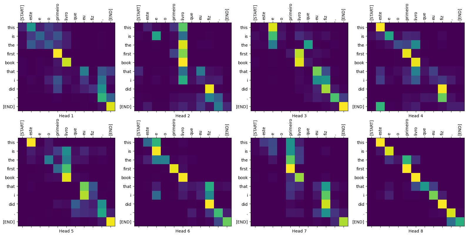
Dikkat çizimleri
Translator sınıfı, modelin dahili çalışmasını görselleştirmek için kullanabileceğiniz bir dikkat haritaları sözlüğü döndürür:
sentence = "este é o primeiro livro que eu fiz."
ground_truth = "this is the first book i've ever done."

translated_text, translated_tokens, attention_weights = translator(
    tf.constant(sentence))
print_translation(sentence, translated_text, ground_truth)
Input:         : este é o primeiro livro que eu fiz.
Prediction     : this is the first book that i did .
Ground truth   : this is the first book i've ever done.
def plot_attention_head(in_tokens, translated_tokens, attention):
  # The plot is of the attention when a token was generated.
  # The model didn't generate `<START>` in the output. Skip it.
  translated_tokens = translated_tokens[1:]

  ax = plt.gca()
  ax.matshow(attention)
  ax.set_xticks(range(len(in_tokens)))
  ax.set_yticks(range(len(translated_tokens)))

  labels = [label.decode('utf-8') for label in in_tokens.numpy()]
  ax.set_xticklabels(
      labels, rotation=90)

  labels = [label.decode('utf-8') for label in translated_tokens.numpy()]
  ax.set_yticklabels(labels)
head = 0
# shape: (batch=1, num_heads, seq_len_q, seq_len_k)
attention_heads = tf.squeeze(
  attention_weights['decoder_layer4_block2'], 0)
attention = attention_heads[head]
attention.shape
TensorShape([10, 11])
in_tokens = tf.convert_to_tensor([sentence])
in_tokens = tokenizers.pt.tokenize(in_tokens).to_tensor()
in_tokens = tokenizers.pt.lookup(in_tokens)[0]
in_tokens
<tf.Tensor: shape=(11,), dtype=string, numpy=
array([b'[START]', b'este', b'e', b'o', b'primeiro', b'livro', b'que',
       b'eu', b'fiz', b'.', b'[END]'], dtype=object)>
translated_tokens
<tf.Tensor: shape=(11,), dtype=string, numpy=
array([b'[START]', b'this', b'is', b'the', b'first', b'book', b'that',
       b'i', b'did', b'.', b'[END]'], dtype=object)>
plot_attention_head(in_tokens, translated_tokens, attention)

def plot_attention_weights(sentence, translated_tokens, attention_heads):
  in_tokens = tf.convert_to_tensor([sentence])
  in_tokens = tokenizers.pt.tokenize(in_tokens).to_tensor()
  in_tokens = tokenizers.pt.lookup(in_tokens)[0]
  in_tokens

  fig = plt.figure(figsize=(16, 8))

  for h, head in enumerate(attention_heads):
    ax = fig.add_subplot(2, 4, h+1)

    plot_attention_head(in_tokens, translated_tokens, head)

    ax.set_xlabel(f'Head {h+1}')

  plt.tight_layout()
  plt.show()
plot_attention_weights(sentence, translated_tokens,
                       attention_weights['decoder_layer4_block2'][0])

Model, bilinmeyen kelimelerde iyi sonuç veriyor. Girdi veri setinde ne "triceratops" ne de "ansiklopedi" yoktur ve model, paylaşılan bir kelime dağarcığı olmasa bile, neredeyse onları çevirmeyi öğrenir:
sentence = "Eu li sobre triceratops na enciclopédia."
ground_truth = "I read about triceratops in the encyclopedia."

translated_text, translated_tokens, attention_weights = translator(
    tf.constant(sentence))
print_translation(sentence, translated_text, ground_truth)

plot_attention_weights(sentence, translated_tokens,
                       attention_weights['decoder_layer4_block2'][0])
Input:         : Eu li sobre triceratops na enciclopédia.
Prediction     : i read about trigatotys in the encyclopedia .
Ground truth   : I read about triceratops in the encyclopedia.

İhracat
Bu çıkarım modeli çalışıyor, bundan sonra onu tf.saved_model olarak dışa aktaracaksınız.
Bunu yapmak için, bu sefer __call__ yönteminde bir tf.function ile başka bir tf.Module alt sınıfına sarın:
class ExportTranslator(tf.Module):
  def __init__(self, translator):
    self.translator = translator

  @tf.function(input_signature=[tf.TensorSpec(shape=[], dtype=tf.string)])
  def __call__(self, sentence):
    (result,
     tokens,
     attention_weights) = self.translator(sentence, max_length=100)

    return result
Yukarıdaki tf.function sadece çıktı cümlesi döndürülür. tf.function içindeki katı olmayan yürütme sayesinde, gereksiz değerler asla hesaplanmaz.
translator = ExportTranslator(translator)
Model, tf.argmax kullanarak tahminlerin kodunu çözdüğünden, tahminler deterministiktir. Orijinal model ve SavedModel yeniden yüklenen model aynı tahminleri vermelidir:
translator("este é o primeiro livro que eu fiz.").numpy()
b'this is the first book that i did .'
tf.saved_model.save(translator, export_dir='translator')
2022-02-04 13:19:17.308292: W tensorflow/python/util/util.cc:368] Sets are not currently considered sequences, but this may change in the future, so consider avoiding using them.
WARNING:absl:Found untraced functions such as embedding_4_layer_call_fn, embedding_4_layer_call_and_return_conditional_losses, dropout_37_layer_call_fn, dropout_37_layer_call_and_return_conditional_losses, embedding_5_layer_call_fn while saving (showing 5 of 224). These functions will not be directly callable after loading.
reloaded = tf.saved_model.load('translator')
reloaded("este é o primeiro livro que eu fiz.").numpy()
b'this is the first book that i did .'
Özet
Bu öğreticide konumsal kodlama, çok kafalı dikkat, maskelemenin önemi ve bir transformatörün nasıl oluşturulacağını öğrendiniz.
Transformatörü eğitmek için farklı bir veri kümesi kullanmayı deneyin. Yukarıdaki hiperparametreleri değiştirerek temel transformatörü veya transformatör XL'yi de oluşturabilirsiniz. BERT oluşturmak ve son model modelleri eğitmek için burada tanımlanan katmanları da kullanabilirsiniz. Ayrıca, daha iyi tahminler elde etmek için ışın aramayı uygulayabilirsiniz.