
| | |  Xem nguồn trên GitHub Xem nguồn trên GitHub |
Hướng dẫn này đào tạo mô hình Transformer để dịch tập dữ liệu từ tiếng Bồ Đào Nha sang tiếng Anh . Đây là một ví dụ nâng cao giả định kiến thức về tạo và chú ý văn bản.
Ý tưởng cốt lõi đằng sau mô hình Máy biến áp là khả năng tự chú ý — khả năng chú ý đến các vị trí khác nhau của trình tự đầu vào để tính toán biểu diễn của trình tự đó. Transformer tạo ra các lớp tự chú ý và được giải thích bên dưới trong các phần Chú ý sản phẩm chấm theo tỷ lệ và Chú ý nhiều đầu .
Một mô hình máy biến áp xử lý đầu vào có kích thước thay đổi bằng cách sử dụng các lớp tự chú ý thay vì RNN hoặc CNN . Kiến trúc chung này có một số ưu điểm:
- Nó không đưa ra giả định về các mối quan hệ thời gian / không gian trên dữ liệu. Điều này là lý tưởng để xử lý một tập hợp các đối tượng (ví dụ, các đơn vị StarCraft ).
- Kết quả đầu ra của lớp có thể được tính toán song song, thay vì một chuỗi như RNN.
- Các mục ở xa có thể ảnh hưởng đến đầu ra của nhau mà không cần chuyển qua nhiều bước RNN, hoặc các lớp tích chập (xem Ví dụ: xem Bộ biến đổi bộ nhớ cảnh ).
- Nó có thể học các phụ thuộc tầm xa. Đây là một thách thức trong nhiều nhiệm vụ trình tự.
Nhược điểm của kiến trúc này là:
- Đối với chuỗi thời gian, đầu ra cho một bước thời gian được tính toán từ toàn bộ lịch sử thay vì chỉ các đầu vào và trạng thái ẩn hiện tại. Điều này có thể kém hiệu quả hơn.
- Nếu đầu vào có mối quan hệ thời gian / không gian, chẳng hạn như văn bản, thì một số mã hóa vị trí phải được thêm vào nếu không mô hình sẽ nhìn thấy một cách hiệu quả một túi từ.
Sau khi huấn luyện mô hình trong sổ tay này, bạn sẽ có thể nhập một câu tiếng Bồ Đào Nha và gửi lại bản dịch tiếng Anh.
Thành lập
pip install tensorflow_datasetspip install -U tensorflow-text
import collections
import logging
import os
import pathlib
import re
import string
import sys
import time

import numpy as np
import matplotlib.pyplot as plt

import tensorflow_datasets as tfds
import tensorflow_text as text
import tensorflow as tf
logging.getLogger('tensorflow').setLevel(logging.ERROR) # suppress warnings
Tải xuống tập dữ liệu
Sử dụng bộ dữ liệu TensorFlow để tải bộ dữ liệu dịch tiếng Bồ Đào Nha-Anh từ Dự án dịch mở TED Talks .
Tập dữ liệu này chứa khoảng 50000 ví dụ đào tạo, 1100 ví dụ xác thực và 2000 ví dụ kiểm tra.
examples, metadata = tfds.load('ted_hrlr_translate/pt_to_en', with_info=True,
                               as_supervised=True)
train_examples, val_examples = examples['train'], examples['validation']
Đối tượng tf.data.Dataset được trả về bởi tập dữ liệu TensorFlow mang lại các cặp ví dụ văn bản:
for pt_examples, en_examples in train_examples.batch(3).take(1):
  for pt in pt_examples.numpy():
    print(pt.decode('utf-8'))

  print()

  for en in en_examples.numpy():
    print(en.decode('utf-8'))
e quando melhoramos a procura , tiramos a única vantagem da impressão , que é a serendipidade .
mas e se estes fatores fossem ativos ?
mas eles não tinham a curiosidade de me testar .

and when you improve searchability , you actually take away the one advantage of print , which is serendipity .
but what if it were active ?
but they did n't test for curiosity .
Mã hóa và tách văn bản
Bạn không thể đào tạo một mô hình trực tiếp trên văn bản. Trước tiên, văn bản cần được chuyển đổi thành một số biểu diễn số. Thông thường, bạn chuyển đổi văn bản thành chuỗi ID mã thông báo, được sử dụng làm chỉ số thành một bản nhúng.
Một cách triển khai phổ biến được trình bày trong hướng dẫn tạo mã định danh từ phụ là xây dựng bộ tạo mã từ khóa phụ ( text.BertTokenizer ) được tối ưu hóa cho tập dữ liệu này và xuất chúng trong một kiểu mẫu đã lưu .
Tải xuống và giải nén và nhập mẫu saved_model :
model_name = "ted_hrlr_translate_pt_en_converter"
tf.keras.utils.get_file(
    f"{model_name}.zip",
    f"https://storage.googleapis.com/download.tensorflow.org/models/{model_name}.zip",
    cache_dir='.', cache_subdir='', extract=True
)
Downloading data from https://storage.googleapis.com/download.tensorflow.org/models/ted_hrlr_translate_pt_en_converter.zip
188416/184801 [==============================] - 0s 0us/step
196608/184801 [===============================] - 0s 0us/step
'./ted_hrlr_translate_pt_en_converter.zip'
tokenizers = tf.saved_model.load(model_name)
tf.saved_model chứa hai văn bản tokenizer, một cho tiếng Anh và một cho tiếng Bồ Đào Nha. Cả hai đều có các phương pháp giống nhau:
[item for item in dir(tokenizers.en) if not item.startswith('_')]
['detokenize',
 'get_reserved_tokens',
 'get_vocab_path',
 'get_vocab_size',
 'lookup',
 'tokenize',
 'tokenizer',
 'vocab']
Phương thức tokenize hóa chuyển đổi một loạt chuỗi thành một loạt ID mã thông báo được đệm. Phương pháp này tách dấu câu, chữ thường và unicode-chuẩn hóa đầu vào trước khi mã hóa. Sự chuẩn hóa đó không hiển thị ở đây vì dữ liệu đầu vào đã được chuẩn hóa.
for en in en_examples.numpy():
  print(en.decode('utf-8'))
and when you improve searchability , you actually take away the one advantage of print , which is serendipity .
but what if it were active ?
but they did n't test for curiosity .
encoded = tokenizers.en.tokenize(en_examples)

for row in encoded.to_list():
  print(row)
[2, 72, 117, 79, 1259, 1491, 2362, 13, 79, 150, 184, 311, 71, 103, 2308, 74, 2679, 13, 148, 80, 55, 4840, 1434, 2423, 540, 15, 3]
[2, 87, 90, 107, 76, 129, 1852, 30, 3]
[2, 87, 83, 149, 50, 9, 56, 664, 85, 2512, 15, 3]
Phương thức detokenize cố gắng chuyển đổi các ID mã thông báo này trở lại thành văn bản có thể đọc được của con người:
round_trip = tokenizers.en.detokenize(encoded)
for line in round_trip.numpy():
  print(line.decode('utf-8'))
and when you improve searchability , you actually take away the one advantage of print , which is serendipity .
but what if it were active ?
but they did n ' t test for curiosity .
Phương pháp lookup cấp thấp hơn chuyển đổi từ mã thông báo-ID thành văn bản mã thông báo:
tokens = tokenizers.en.lookup(encoded)
tokens
<tf.RaggedTensor [[b'[START]', b'and', b'when', b'you', b'improve', b'search', b'##ability',
  b',', b'you', b'actually', b'take', b'away', b'the', b'one', b'advantage',
  b'of', b'print', b',', b'which', b'is', b's', b'##ere', b'##nd', b'##ip',
  b'##ity', b'.', b'[END]']                                                 ,
 [b'[START]', b'but', b'what', b'if', b'it', b'were', b'active', b'?',
  b'[END]']                                                           ,
 [b'[START]', b'but', b'they', b'did', b'n', b"'", b't', b'test', b'for',
  b'curiosity', b'.', b'[END]']                                          ]>
Ở đây bạn có thể thấy khía cạnh "subword" của tokenizers. Từ "khả năng tìm kiếm" được phân tách thành "khả năng tìm kiếm ##" và từ "khả năng tìm kiếm" thành "s ##rect ## nd ## ip ## ity"
Thiết lập đường dẫn đầu vào
Để xây dựng một đường dẫn đầu vào phù hợp cho việc đào tạo, bạn sẽ áp dụng một số biến đổi cho tập dữ liệu.
Hàm này sẽ được sử dụng để mã hóa các lô văn bản thô:
def tokenize_pairs(pt, en):
    pt = tokenizers.pt.tokenize(pt)
    # Convert from ragged to dense, padding with zeros.
    pt = pt.to_tensor()

    en = tokenizers.en.tokenize(en)
    # Convert from ragged to dense, padding with zeros.
    en = en.to_tensor()
    return pt, en
Đây là một đường dẫn đầu vào đơn giản có thể xử lý, xáo trộn và phân lô dữ liệu:
BUFFER_SIZE = 20000
BATCH_SIZE = 64
def make_batches(ds):
  return (
      ds
      .cache()
      .shuffle(BUFFER_SIZE)
      .batch(BATCH_SIZE)
      .map(tokenize_pairs, num_parallel_calls=tf.data.AUTOTUNE)
      .prefetch(tf.data.AUTOTUNE))


train_batches = make_batches(train_examples)
val_batches = make_batches(val_examples)
Mã hóa vị trí
Các lớp chú ý xem đầu vào của chúng là một tập hợp các vectơ, không có thứ tự tuần tự. Mô hình này cũng không chứa bất kỳ lớp lặp lại hoặc tích tụ nào. Do đó, một "mã hóa vị trí" được thêm vào để cung cấp cho mô hình một số thông tin về vị trí tương đối của các thẻ trong câu.
Vectơ mã hóa vị trí được thêm vào vectơ nhúng. Nhúng đại diện cho một mã thông báo trong không gian d chiều nơi các mã thông báo có ý nghĩa tương tự sẽ gần nhau hơn. Nhưng các nhúng không mã hóa vị trí tương đối của các mã thông báo trong một câu. Vì vậy, sau khi thêm mã hóa vị trí, các mã thông báo sẽ gần nhau hơn dựa trên sự giống nhau về ý nghĩa của chúng và vị trí của chúng trong câu , trong không gian d chiều.
Công thức tính toán mã hóa vị trí như sau:
\[\Large{PE_{(pos, 2i)} = \sin(pos / 10000^{2i / d_{model} })} \]
\[\Large{PE_{(pos, 2i+1)} = \cos(pos / 10000^{2i / d_{model} })} \]
def get_angles(pos, i, d_model):
  angle_rates = 1 / np.power(10000, (2 * (i//2)) / np.float32(d_model))
  return pos * angle_rates
def positional_encoding(position, d_model):
  angle_rads = get_angles(np.arange(position)[:, np.newaxis],
                          np.arange(d_model)[np.newaxis, :],
                          d_model)

  # apply sin to even indices in the array; 2i
  angle_rads[:, 0::2] = np.sin(angle_rads[:, 0::2])

  # apply cos to odd indices in the array; 2i+1
  angle_rads[:, 1::2] = np.cos(angle_rads[:, 1::2])

  pos_encoding = angle_rads[np.newaxis, ...]

  return tf.cast(pos_encoding, dtype=tf.float32)
n, d = 2048, 512
pos_encoding = positional_encoding(n, d)
print(pos_encoding.shape)
pos_encoding = pos_encoding[0]

# Juggle the dimensions for the plot
pos_encoding = tf.reshape(pos_encoding, (n, d//2, 2))
pos_encoding = tf.transpose(pos_encoding, (2, 1, 0))
pos_encoding = tf.reshape(pos_encoding, (d, n))

plt.pcolormesh(pos_encoding, cmap='RdBu')
plt.ylabel('Depth')
plt.xlabel('Position')
plt.colorbar()
plt.show()
(1, 2048, 512)

Đắp mặt nạ
Che dấu tất cả các mã thông báo pad trong một loạt chuỗi. Nó đảm bảo rằng mô hình không coi padding là đầu vào. Mặt nạ cho biết vị trí có giá trị pad 0 : nó xuất ra giá trị 1 tại các vị trí đó và 0 nếu không.
def create_padding_mask(seq):
  seq = tf.cast(tf.math.equal(seq, 0), tf.float32)

  # add extra dimensions to add the padding
  # to the attention logits.
  return seq[:, tf.newaxis, tf.newaxis, :]  # (batch_size, 1, 1, seq_len)
x = tf.constant([[7, 6, 0, 0, 1], [1, 2, 3, 0, 0], [0, 0, 0, 4, 5]])
create_padding_mask(x)
<tf.Tensor: shape=(3, 1, 1, 5), dtype=float32, numpy=
array([[[[0., 0., 1., 1., 0.]]],


       [[[0., 0., 0., 1., 1.]]],


       [[[1., 1., 1., 0., 0.]]]], dtype=float32)>
Mặt nạ nhìn trước được sử dụng để che dấu các mã thông báo trong tương lai theo một trình tự. Nói cách khác, mặt nạ cho biết mục nào không nên được sử dụng.
Điều này có nghĩa là để dự đoán mã thông báo thứ ba, chỉ mã thông báo đầu tiên và thứ hai sẽ được sử dụng. Tương tự như vậy để dự đoán mã thông báo thứ tư, chỉ mã thông báo đầu tiên, thứ hai và thứ ba sẽ được sử dụng, v.v.
def create_look_ahead_mask(size):
  mask = 1 - tf.linalg.band_part(tf.ones((size, size)), -1, 0)
  return mask  # (seq_len, seq_len)
x = tf.random.uniform((1, 3))
temp = create_look_ahead_mask(x.shape[1])
temp
<tf.Tensor: shape=(3, 3), dtype=float32, numpy=
array([[0., 1., 1.],
       [0., 0., 1.],
       [0., 0., 0.]], dtype=float32)>
Sự chú ý của sản phẩm chấm theo tỷ lệ
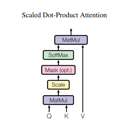
Chức năng chú ý được sử dụng bởi máy biến áp có ba đầu vào: Q (truy vấn), K (phím), V (giá trị). Phương trình được sử dụng để tính toán trọng số chú ý là:
\[\Large{Attention(Q, K, V) = softmax_k\left(\frac{QK^T}{\sqrt{d_k} }\right) V} \]
Sự chú ý của sản phẩm chấm được chia tỷ lệ bằng hệ số căn bậc hai của độ sâu. Điều này được thực hiện bởi vì đối với các giá trị độ sâu lớn, sản phẩm chấm phát triển lớn về độ lớn đẩy hàm softmax ở nơi nó có độ dốc nhỏ dẫn đến softmax rất cứng.
Ví dụ, xem xét rằng Q và K có giá trị trung bình bằng 0 và phương sai là 1. Phép nhân ma trận của chúng sẽ có giá trị trung bình bằng 0 và phương sai là dk . Vì vậy, căn bậc hai của dk được sử dụng để chia tỷ lệ, vì vậy bạn sẽ nhận được một phương sai nhất quán bất kể giá trị của dk . Nếu phương sai quá thấp, đầu ra có thể quá phẳng để tối ưu hóa hiệu quả. Nếu phương sai quá cao, softmax có thể bão hòa khi khởi tạo, gây khó khăn cho việc học.
Mặt nạ được nhân với -1e9 (gần với âm vô cực). Điều này được thực hiện bởi vì mặt nạ được tính tổng với phép nhân ma trận tỷ lệ của Q và K và được áp dụng ngay trước một softmax. Mục tiêu là loại bỏ các ô này và đầu vào âm lớn cho softmax gần bằng 0 trong đầu ra.
def scaled_dot_product_attention(q, k, v, mask):
  """Calculate the attention weights.
  q, k, v must have matching leading dimensions.
  k, v must have matching penultimate dimension, i.e.: seq_len_k = seq_len_v.
  The mask has different shapes depending on its type(padding or look ahead)
  but it must be broadcastable for addition.

  Args:
    q: query shape == (..., seq_len_q, depth)
    k: key shape == (..., seq_len_k, depth)
    v: value shape == (..., seq_len_v, depth_v)
    mask: Float tensor with shape broadcastable
          to (..., seq_len_q, seq_len_k). Defaults to None.

  Returns:
    output, attention_weights
  """

  matmul_qk = tf.matmul(q, k, transpose_b=True)  # (..., seq_len_q, seq_len_k)

  # scale matmul_qk
  dk = tf.cast(tf.shape(k)[-1], tf.float32)
  scaled_attention_logits = matmul_qk / tf.math.sqrt(dk)

  # add the mask to the scaled tensor.
  if mask is not None:
    scaled_attention_logits += (mask * -1e9)

  # softmax is normalized on the last axis (seq_len_k) so that the scores
  # add up to 1.
  attention_weights = tf.nn.softmax(scaled_attention_logits, axis=-1)  # (..., seq_len_q, seq_len_k)

  output = tf.matmul(attention_weights, v)  # (..., seq_len_q, depth_v)

  return output, attention_weights
Khi quá trình chuẩn hóa softmax được thực hiện trên K, các giá trị của nó quyết định mức độ quan trọng đối với Q.
Đầu ra đại diện cho phép nhân của trọng số chú ý và vectơ V (giá trị). Điều này đảm bảo rằng các mã thông báo bạn muốn tập trung vào được giữ nguyên và các mã thông báo không liên quan sẽ bị loại bỏ.
def print_out(q, k, v):
  temp_out, temp_attn = scaled_dot_product_attention(
      q, k, v, None)
  print('Attention weights are:')
  print(temp_attn)
  print('Output is:')
  print(temp_out)
np.set_printoptions(suppress=True)

temp_k = tf.constant([[10, 0, 0],
                      [0, 10, 0],
                      [0, 0, 10],
                      [0, 0, 10]], dtype=tf.float32)  # (4, 3)

temp_v = tf.constant([[1, 0],
                      [10, 0],
                      [100, 5],
                      [1000, 6]], dtype=tf.float32)  # (4, 2)

# This `query` aligns with the second `key`,
# so the second `value` is returned.
temp_q = tf.constant([[0, 10, 0]], dtype=tf.float32)  # (1, 3)
print_out(temp_q, temp_k, temp_v)
Attention weights are:
tf.Tensor([[0. 1. 0. 0.]], shape=(1, 4), dtype=float32)
Output is:
tf.Tensor([[10.  0.]], shape=(1, 2), dtype=float32)
# This query aligns with a repeated key (third and fourth),
# so all associated values get averaged.
temp_q = tf.constant([[0, 0, 10]], dtype=tf.float32)  # (1, 3)
print_out(temp_q, temp_k, temp_v)
Attention weights are:
tf.Tensor([[0.  0.  0.5 0.5]], shape=(1, 4), dtype=float32)
Output is:
tf.Tensor([[550.    5.5]], shape=(1, 2), dtype=float32)
# This query aligns equally with the first and second key,
# so their values get averaged.
temp_q = tf.constant([[10, 10, 0]], dtype=tf.float32)  # (1, 3)
print_out(temp_q, temp_k, temp_v)
Attention weights are:
tf.Tensor([[0.5 0.5 0.  0. ]], shape=(1, 4), dtype=float32)
Output is:
tf.Tensor([[5.5 0. ]], shape=(1, 2), dtype=float32)
Vượt qua tất cả các truy vấn cùng nhau.
temp_q = tf.constant([[0, 0, 10],
                      [0, 10, 0],
                      [10, 10, 0]], dtype=tf.float32)  # (3, 3)
print_out(temp_q, temp_k, temp_v)
Attention weights are:
tf.Tensor(
[[0.  0.  0.5 0.5]
 [0.  1.  0.  0. ]
 [0.5 0.5 0.  0. ]], shape=(3, 4), dtype=float32)
Output is:
tf.Tensor(
[[550.    5.5]
 [ 10.    0. ]
 [  5.5   0. ]], shape=(3, 2), dtype=float32)
Sự chú ý từ nhiều phía
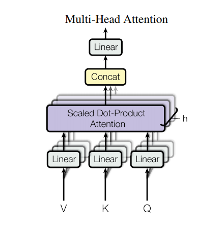
Sự chú ý đa đầu bao gồm bốn phần:
- Các lớp tuyến tính.
- Sự chú ý theo tỷ lệ chấm-sản phẩm.
- Lớp tuyến tính cuối cùng.
Mỗi khối chú ý nhiều đầu nhận được ba đầu vào; Q (truy vấn), K (khóa), V (giá trị). Chúng được đưa qua các lớp tuyến tính (Dày đặc) trước chức năng chú ý nhiều đầu.
Trong sơ đồ trên (K,Q,V) được chuyển qua các lớp tuyến tính riêng biệt ( Dense ) cho mỗi đầu chú ý. Để đơn giản / hiệu quả, đoạn mã dưới đây thực hiện điều này bằng cách sử dụng một lớp dày đặc duy nhất với số đầu ra num_heads nhiều lần số đầu ra. Đầu ra được sắp xếp lại thành hình dạng của (batch, num_heads, ...) trước khi áp dụng hàm chú ý.
Hàm scaled_dot_product_attention được định nghĩa ở trên được áp dụng trong một lệnh gọi duy nhất, được phát sóng để đạt hiệu quả. Trong bước chú ý phải sử dụng mặt nạ thích hợp. Đầu ra chú ý cho mỗi phần đầu sau đó được nối (sử dụng tf.transpose và tf.reshape ) và đưa qua một lớp Dense cuối cùng.
Thay vì một đầu chú ý duy nhất, Q, K và V được chia thành nhiều đầu vì nó cho phép mô hình cùng tham gia vào thông tin từ các không gian con biểu diễn khác nhau ở các vị trí khác nhau. Sau khi tách, mỗi phần đầu có số chiều giảm, do đó, tổng chi phí tính toán giống như sự chú ý của phần đầu duy nhất với kích thước đầy đủ.
class MultiHeadAttention(tf.keras.layers.Layer):
  def __init__(self, d_model, num_heads):
    super(MultiHeadAttention, self).__init__()
    self.num_heads = num_heads
    self.d_model = d_model

    assert d_model % self.num_heads == 0

    self.depth = d_model // self.num_heads

    self.wq = tf.keras.layers.Dense(d_model)
    self.wk = tf.keras.layers.Dense(d_model)
    self.wv = tf.keras.layers.Dense(d_model)

    self.dense = tf.keras.layers.Dense(d_model)

  def split_heads(self, x, batch_size):
    """Split the last dimension into (num_heads, depth).
    Transpose the result such that the shape is (batch_size, num_heads, seq_len, depth)
    """
    x = tf.reshape(x, (batch_size, -1, self.num_heads, self.depth))
    return tf.transpose(x, perm=[0, 2, 1, 3])

  def call(self, v, k, q, mask):
    batch_size = tf.shape(q)[0]

    q = self.wq(q)  # (batch_size, seq_len, d_model)
    k = self.wk(k)  # (batch_size, seq_len, d_model)
    v = self.wv(v)  # (batch_size, seq_len, d_model)

    q = self.split_heads(q, batch_size)  # (batch_size, num_heads, seq_len_q, depth)
    k = self.split_heads(k, batch_size)  # (batch_size, num_heads, seq_len_k, depth)
    v = self.split_heads(v, batch_size)  # (batch_size, num_heads, seq_len_v, depth)

    # scaled_attention.shape == (batch_size, num_heads, seq_len_q, depth)
    # attention_weights.shape == (batch_size, num_heads, seq_len_q, seq_len_k)
    scaled_attention, attention_weights = scaled_dot_product_attention(
        q, k, v, mask)

    scaled_attention = tf.transpose(scaled_attention, perm=[0, 2, 1, 3])  # (batch_size, seq_len_q, num_heads, depth)

    concat_attention = tf.reshape(scaled_attention,
                                  (batch_size, -1, self.d_model))  # (batch_size, seq_len_q, d_model)

    output = self.dense(concat_attention)  # (batch_size, seq_len_q, d_model)

    return output, attention_weights
Tạo một lớp MultiHeadAttention để dùng thử. Tại mỗi vị trí trong chuỗi, y , MultiHeadAttention chạy tất cả 8 đầu chú ý trên tất cả các vị trí khác trong chuỗi, trả về một vectơ mới có cùng độ dài tại mỗi vị trí.
temp_mha = MultiHeadAttention(d_model=512, num_heads=8)
y = tf.random.uniform((1, 60, 512))  # (batch_size, encoder_sequence, d_model)
out, attn = temp_mha(y, k=y, q=y, mask=None)
out.shape, attn.shape
(TensorShape([1, 60, 512]), TensorShape([1, 8, 60, 60]))
Điểm mạng chuyển tiếp nguồn cấp dữ liệu khôn ngoan
Mạng chuyển tiếp nguồn cấp dữ liệu khôn ngoan bao gồm hai lớp được kết nối đầy đủ với kích hoạt ReLU ở giữa.
def point_wise_feed_forward_network(d_model, dff):
  return tf.keras.Sequential([
      tf.keras.layers.Dense(dff, activation='relu'),  # (batch_size, seq_len, dff)
      tf.keras.layers.Dense(d_model)  # (batch_size, seq_len, d_model)
  ])
sample_ffn = point_wise_feed_forward_network(512, 2048)
sample_ffn(tf.random.uniform((64, 50, 512))).shape
TensorShape([64, 50, 512])
Bộ mã hóa và giải mã
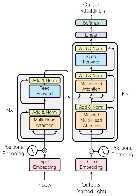
Mô hình máy biến áp tuân theo cùng một mô hình chung như một trình tự tiêu chuẩn để trình tự với mô hình chú ý .
- Câu đầu vào được chuyển qua
Nlớp mã hóa tạo ra kết quả đầu ra cho mỗi mã thông báo trong chuỗi. - Bộ giải mã chú ý đến đầu ra của bộ mã hóa và đầu vào của chính nó (tự chú ý) để dự đoán từ tiếp theo.
Lớp mã hóa
Mỗi lớp mã hóa bao gồm các lớp con:
- Chú ý nhiều đầu (với mặt nạ đệm)
- Chỉ ra các mạng chuyển tiếp nguồn cấp dữ liệu khôn ngoan.
Mỗi lớp con này có một kết nối dư xung quanh nó, theo sau là chuẩn hóa lớp. Các kết nối dư giúp tránh vấn đề độ dốc biến mất trong các mạng sâu.
Đầu ra của mỗi lớp con là LayerNorm(x + Sublayer(x)) . Quá trình chuẩn hóa được thực hiện trên d_model (cuối cùng). Có N lớp mã hóa trong máy biến áp.
class EncoderLayer(tf.keras.layers.Layer):
  def __init__(self, d_model, num_heads, dff, rate=0.1):
    super(EncoderLayer, self).__init__()

    self.mha = MultiHeadAttention(d_model, num_heads)
    self.ffn = point_wise_feed_forward_network(d_model, dff)

    self.layernorm1 = tf.keras.layers.LayerNormalization(epsilon=1e-6)
    self.layernorm2 = tf.keras.layers.LayerNormalization(epsilon=1e-6)

    self.dropout1 = tf.keras.layers.Dropout(rate)
    self.dropout2 = tf.keras.layers.Dropout(rate)

  def call(self, x, training, mask):

    attn_output, _ = self.mha(x, x, x, mask)  # (batch_size, input_seq_len, d_model)
    attn_output = self.dropout1(attn_output, training=training)
    out1 = self.layernorm1(x + attn_output)  # (batch_size, input_seq_len, d_model)

    ffn_output = self.ffn(out1)  # (batch_size, input_seq_len, d_model)
    ffn_output = self.dropout2(ffn_output, training=training)
    out2 = self.layernorm2(out1 + ffn_output)  # (batch_size, input_seq_len, d_model)

    return out2
sample_encoder_layer = EncoderLayer(512, 8, 2048)

sample_encoder_layer_output = sample_encoder_layer(
    tf.random.uniform((64, 43, 512)), False, None)

sample_encoder_layer_output.shape  # (batch_size, input_seq_len, d_model)
TensorShape([64, 43, 512])
Lớp giải mã
Mỗi lớp bộ giải mã bao gồm các lớp con:
- Mặt nạ chú ý nhiều đầu (với mặt nạ nhìn trước và mặt nạ đệm)
- Chú ý nhiều đầu (có đệm mặt nạ). V (giá trị) và K (phím) nhận đầu ra bộ mã hóa làm đầu vào. Q (truy vấn) nhận kết quả đầu ra từ lớp con chú ý nhiều đầu có mặt nạ.
- Chỉ ra các mạng chuyển tiếp nguồn cấp dữ liệu khôn ngoan
Mỗi lớp con này có một kết nối dư xung quanh nó, theo sau là chuẩn hóa lớp. Đầu ra của mỗi lớp con là LayerNorm(x + Sublayer(x)) . Quá trình chuẩn hóa được thực hiện trên d_model (cuối cùng).
Có N lớp giải mã trong máy biến áp.
Khi Q nhận đầu ra từ khối chú ý đầu tiên của bộ giải mã và K nhận đầu ra của bộ mã hóa, trọng số chú ý thể hiện tầm quan trọng đối với đầu vào của bộ giải mã dựa trên đầu ra của bộ mã hóa. Nói cách khác, bộ giải mã dự đoán mã thông báo tiếp theo bằng cách xem đầu ra của bộ mã hóa và tự tham gia vào đầu ra của chính nó. Xem phần minh họa ở trên trong phần chú ý sản phẩm chấm theo tỷ lệ.
class DecoderLayer(tf.keras.layers.Layer):
  def __init__(self, d_model, num_heads, dff, rate=0.1):
    super(DecoderLayer, self).__init__()

    self.mha1 = MultiHeadAttention(d_model, num_heads)
    self.mha2 = MultiHeadAttention(d_model, num_heads)

    self.ffn = point_wise_feed_forward_network(d_model, dff)

    self.layernorm1 = tf.keras.layers.LayerNormalization(epsilon=1e-6)
    self.layernorm2 = tf.keras.layers.LayerNormalization(epsilon=1e-6)
    self.layernorm3 = tf.keras.layers.LayerNormalization(epsilon=1e-6)

    self.dropout1 = tf.keras.layers.Dropout(rate)
    self.dropout2 = tf.keras.layers.Dropout(rate)
    self.dropout3 = tf.keras.layers.Dropout(rate)

  def call(self, x, enc_output, training,
           look_ahead_mask, padding_mask):
    # enc_output.shape == (batch_size, input_seq_len, d_model)

    attn1, attn_weights_block1 = self.mha1(x, x, x, look_ahead_mask)  # (batch_size, target_seq_len, d_model)
    attn1 = self.dropout1(attn1, training=training)
    out1 = self.layernorm1(attn1 + x)

    attn2, attn_weights_block2 = self.mha2(
        enc_output, enc_output, out1, padding_mask)  # (batch_size, target_seq_len, d_model)
    attn2 = self.dropout2(attn2, training=training)
    out2 = self.layernorm2(attn2 + out1)  # (batch_size, target_seq_len, d_model)

    ffn_output = self.ffn(out2)  # (batch_size, target_seq_len, d_model)
    ffn_output = self.dropout3(ffn_output, training=training)
    out3 = self.layernorm3(ffn_output + out2)  # (batch_size, target_seq_len, d_model)

    return out3, attn_weights_block1, attn_weights_block2
sample_decoder_layer = DecoderLayer(512, 8, 2048)

sample_decoder_layer_output, _, _ = sample_decoder_layer(
    tf.random.uniform((64, 50, 512)), sample_encoder_layer_output,
    False, None, None)

sample_decoder_layer_output.shape  # (batch_size, target_seq_len, d_model)
TensorShape([64, 50, 512])
Mã hoá
Bộ Encoder bao gồm:
- Nhúng đầu vào
- Mã hóa vị trí
- N lớp mã hóa
Đầu vào được đưa qua một phép nhúng được tổng hợp bằng mã hóa vị trí. Đầu ra của tổng kết này là đầu vào cho các lớp mã hóa. Đầu ra của bộ mã hóa là đầu vào cho bộ giải mã.
class Encoder(tf.keras.layers.Layer):
  def __init__(self, num_layers, d_model, num_heads, dff, input_vocab_size,
               maximum_position_encoding, rate=0.1):
    super(Encoder, self).__init__()

    self.d_model = d_model
    self.num_layers = num_layers

    self.embedding = tf.keras.layers.Embedding(input_vocab_size, d_model)
    self.pos_encoding = positional_encoding(maximum_position_encoding,
                                            self.d_model)

    self.enc_layers = [EncoderLayer(d_model, num_heads, dff, rate)
                       for _ in range(num_layers)]

    self.dropout = tf.keras.layers.Dropout(rate)

  def call(self, x, training, mask):

    seq_len = tf.shape(x)[1]

    # adding embedding and position encoding.
    x = self.embedding(x)  # (batch_size, input_seq_len, d_model)
    x *= tf.math.sqrt(tf.cast(self.d_model, tf.float32))
    x += self.pos_encoding[:, :seq_len, :]

    x = self.dropout(x, training=training)

    for i in range(self.num_layers):
      x = self.enc_layers[i](x, training, mask)

    return x  # (batch_size, input_seq_len, d_model)
sample_encoder = Encoder(num_layers=2, d_model=512, num_heads=8,
                         dff=2048, input_vocab_size=8500,
                         maximum_position_encoding=10000)
temp_input = tf.random.uniform((64, 62), dtype=tf.int64, minval=0, maxval=200)

sample_encoder_output = sample_encoder(temp_input, training=False, mask=None)

print(sample_encoder_output.shape)  # (batch_size, input_seq_len, d_model)
(64, 62, 512)
Người giải mã
Bộ Decoder bao gồm:
- Nhúng đầu ra
- Mã hóa vị trí
- N lớp bộ giải mã
Mục tiêu được đưa qua một phép nhúng được tổng hợp bằng mã hóa vị trí. Đầu ra của phép tổng kết này là đầu vào cho các lớp giải mã. Đầu ra của bộ giải mã là đầu vào của lớp tuyến tính cuối cùng.
class Decoder(tf.keras.layers.Layer):
  def __init__(self, num_layers, d_model, num_heads, dff, target_vocab_size,
               maximum_position_encoding, rate=0.1):
    super(Decoder, self).__init__()

    self.d_model = d_model
    self.num_layers = num_layers

    self.embedding = tf.keras.layers.Embedding(target_vocab_size, d_model)
    self.pos_encoding = positional_encoding(maximum_position_encoding, d_model)

    self.dec_layers = [DecoderLayer(d_model, num_heads, dff, rate)
                       for _ in range(num_layers)]
    self.dropout = tf.keras.layers.Dropout(rate)

  def call(self, x, enc_output, training,
           look_ahead_mask, padding_mask):

    seq_len = tf.shape(x)[1]
    attention_weights = {}

    x = self.embedding(x)  # (batch_size, target_seq_len, d_model)
    x *= tf.math.sqrt(tf.cast(self.d_model, tf.float32))
    x += self.pos_encoding[:, :seq_len, :]

    x = self.dropout(x, training=training)

    for i in range(self.num_layers):
      x, block1, block2 = self.dec_layers[i](x, enc_output, training,
                                             look_ahead_mask, padding_mask)

      attention_weights[f'decoder_layer{i+1}_block1'] = block1
      attention_weights[f'decoder_layer{i+1}_block2'] = block2

    # x.shape == (batch_size, target_seq_len, d_model)
    return x, attention_weights
sample_decoder = Decoder(num_layers=2, d_model=512, num_heads=8,
                         dff=2048, target_vocab_size=8000,
                         maximum_position_encoding=5000)
temp_input = tf.random.uniform((64, 26), dtype=tf.int64, minval=0, maxval=200)

output, attn = sample_decoder(temp_input,
                              enc_output=sample_encoder_output,
                              training=False,
                              look_ahead_mask=None,
                              padding_mask=None)

output.shape, attn['decoder_layer2_block2'].shape
(TensorShape([64, 26, 512]), TensorShape([64, 8, 26, 62]))
Tạo máy biến áp
Máy biến áp bao gồm bộ mã hóa, bộ giải mã và một lớp tuyến tính cuối cùng. Đầu ra của bộ giải mã là đầu vào của lớp tuyến tính và đầu ra của nó được trả về.
class Transformer(tf.keras.Model):
  def __init__(self, num_layers, d_model, num_heads, dff, input_vocab_size,
               target_vocab_size, pe_input, pe_target, rate=0.1):
    super().__init__()
    self.encoder = Encoder(num_layers, d_model, num_heads, dff,
                             input_vocab_size, pe_input, rate)

    self.decoder = Decoder(num_layers, d_model, num_heads, dff,
                           target_vocab_size, pe_target, rate)

    self.final_layer = tf.keras.layers.Dense(target_vocab_size)

  def call(self, inputs, training):
    # Keras models prefer if you pass all your inputs in the first argument
    inp, tar = inputs

    enc_padding_mask, look_ahead_mask, dec_padding_mask = self.create_masks(inp, tar)

    enc_output = self.encoder(inp, training, enc_padding_mask)  # (batch_size, inp_seq_len, d_model)

    # dec_output.shape == (batch_size, tar_seq_len, d_model)
    dec_output, attention_weights = self.decoder(
        tar, enc_output, training, look_ahead_mask, dec_padding_mask)

    final_output = self.final_layer(dec_output)  # (batch_size, tar_seq_len, target_vocab_size)

    return final_output, attention_weights

  def create_masks(self, inp, tar):
    # Encoder padding mask
    enc_padding_mask = create_padding_mask(inp)

    # Used in the 2nd attention block in the decoder.
    # This padding mask is used to mask the encoder outputs.
    dec_padding_mask = create_padding_mask(inp)

    # Used in the 1st attention block in the decoder.
    # It is used to pad and mask future tokens in the input received by
    # the decoder.
    look_ahead_mask = create_look_ahead_mask(tf.shape(tar)[1])
    dec_target_padding_mask = create_padding_mask(tar)
    look_ahead_mask = tf.maximum(dec_target_padding_mask, look_ahead_mask)

    return enc_padding_mask, look_ahead_mask, dec_padding_mask
sample_transformer = Transformer(
    num_layers=2, d_model=512, num_heads=8, dff=2048,
    input_vocab_size=8500, target_vocab_size=8000,
    pe_input=10000, pe_target=6000)

temp_input = tf.random.uniform((64, 38), dtype=tf.int64, minval=0, maxval=200)
temp_target = tf.random.uniform((64, 36), dtype=tf.int64, minval=0, maxval=200)

fn_out, _ = sample_transformer([temp_input, temp_target], training=False)

fn_out.shape  # (batch_size, tar_seq_len, target_vocab_size)
TensorShape([64, 36, 8000])
Đặt siêu tham số
Để giữ cho ví dụ này nhỏ và tương đối nhanh, các giá trị cho num_layers, d_model, dff đã được giảm bớt.
Mô hình cơ sở được mô tả trong bài báo được sử dụng: num_layers=6, d_model=512, dff=2048 .
num_layers = 4
d_model = 128
dff = 512
num_heads = 8
dropout_rate = 0.1
Trình tối ưu hóa
Sử dụng trình tối ưu hóa Adam với công cụ lập lịch tốc độ học tập tùy chỉnh theo công thức trong bài báo .
\[\Large{lrate = d_{model}^{-0.5} * \min(step{\_}num^{-0.5}, step{\_}num \cdot warmup{\_}steps^{-1.5})}\]
class CustomSchedule(tf.keras.optimizers.schedules.LearningRateSchedule):
  def __init__(self, d_model, warmup_steps=4000):
    super(CustomSchedule, self).__init__()

    self.d_model = d_model
    self.d_model = tf.cast(self.d_model, tf.float32)

    self.warmup_steps = warmup_steps

  def __call__(self, step):
    arg1 = tf.math.rsqrt(step)
    arg2 = step * (self.warmup_steps ** -1.5)

    return tf.math.rsqrt(self.d_model) * tf.math.minimum(arg1, arg2)
learning_rate = CustomSchedule(d_model)

optimizer = tf.keras.optimizers.Adam(learning_rate, beta_1=0.9, beta_2=0.98,
                                     epsilon=1e-9)
temp_learning_rate_schedule = CustomSchedule(d_model)

plt.plot(temp_learning_rate_schedule(tf.range(40000, dtype=tf.float32)))
plt.ylabel("Learning Rate")
plt.xlabel("Train Step")
Text(0.5, 0, 'Train Step')

Mất mát và số liệu
Vì các chuỗi mục tiêu được đệm, điều quan trọng là phải áp dụng mặt nạ đệm khi tính toán tổn thất.
loss_object = tf.keras.losses.SparseCategoricalCrossentropy(
    from_logits=True, reduction='none')
def loss_function(real, pred):
  mask = tf.math.logical_not(tf.math.equal(real, 0))
  loss_ = loss_object(real, pred)

  mask = tf.cast(mask, dtype=loss_.dtype)
  loss_ *= mask

  return tf.reduce_sum(loss_)/tf.reduce_sum(mask)


def accuracy_function(real, pred):
  accuracies = tf.equal(real, tf.argmax(pred, axis=2))

  mask = tf.math.logical_not(tf.math.equal(real, 0))
  accuracies = tf.math.logical_and(mask, accuracies)

  accuracies = tf.cast(accuracies, dtype=tf.float32)
  mask = tf.cast(mask, dtype=tf.float32)
  return tf.reduce_sum(accuracies)/tf.reduce_sum(mask)
train_loss = tf.keras.metrics.Mean(name='train_loss')
train_accuracy = tf.keras.metrics.Mean(name='train_accuracy')
Đào tạo và kiểm tra
transformer = Transformer(
    num_layers=num_layers,
    d_model=d_model,
    num_heads=num_heads,
    dff=dff,
    input_vocab_size=tokenizers.pt.get_vocab_size().numpy(),
    target_vocab_size=tokenizers.en.get_vocab_size().numpy(),
    pe_input=1000,
    pe_target=1000,
    rate=dropout_rate)
Tạo đường dẫn điểm kiểm tra và trình quản lý điểm kiểm tra. Điều này sẽ được sử dụng để lưu các điểm kiểm tra mỗi n kỷ nguyên.
checkpoint_path = "./checkpoints/train"

ckpt = tf.train.Checkpoint(transformer=transformer,
                           optimizer=optimizer)

ckpt_manager = tf.train.CheckpointManager(ckpt, checkpoint_path, max_to_keep=5)

# if a checkpoint exists, restore the latest checkpoint.
if ckpt_manager.latest_checkpoint:
  ckpt.restore(ckpt_manager.latest_checkpoint)
  print('Latest checkpoint restored!!')
Mục tiêu được chia thành tar_inp và tar_real. tar_inp được chuyển như một đầu vào cho bộ giải mã. tar_real là cùng một đầu vào được dịch chuyển bằng 1: Tại mỗi vị trí trong tar_input , tar_real chứa mã thông báo tiếp theo cần được dự đoán.
Ví dụ, sentence = "SOS Một con sư tử trong rừng đang ngủ EOS"
tar_inp = "SOS Một con sư tử trong rừng đang ngủ"
tar_real = "Một con sư tử trong rừng đang ngủ EOS"
Máy biến áp là một mô hình tự động hồi quy: nó đưa ra dự đoán từng phần một và sử dụng kết quả đầu ra của nó cho đến nay để quyết định phải làm gì tiếp theo.
Trong quá trình đào tạo, ví dụ này sử dụng giáo viên ép buộc (giống như trong hướng dẫn tạo văn bản ). Giáo viên buộc phải chuyển đầu ra thực sự cho bước thời gian tiếp theo bất kể mô hình dự đoán những gì ở bước thời gian hiện tại.
Khi máy biến áp dự đoán từng mã thông báo, khả năng tự chú ý cho phép nó xem xét các mã thông báo trước đó trong trình tự đầu vào để dự đoán tốt hơn mã thông báo tiếp theo.
Để ngăn mô hình nhìn trộm đầu ra dự kiến, mô hình sử dụng mặt nạ nhìn trước.
EPOCHS = 20
# The @tf.function trace-compiles train_step into a TF graph for faster
# execution. The function specializes to the precise shape of the argument
# tensors. To avoid re-tracing due to the variable sequence lengths or variable
# batch sizes (the last batch is smaller), use input_signature to specify
# more generic shapes.

train_step_signature = [
    tf.TensorSpec(shape=(None, None), dtype=tf.int64),
    tf.TensorSpec(shape=(None, None), dtype=tf.int64),
]


@tf.function(input_signature=train_step_signature)
def train_step(inp, tar):
  tar_inp = tar[:, :-1]
  tar_real = tar[:, 1:]

  with tf.GradientTape() as tape:
    predictions, _ = transformer([inp, tar_inp],
                                 training = True)
    loss = loss_function(tar_real, predictions)

  gradients = tape.gradient(loss, transformer.trainable_variables)
  optimizer.apply_gradients(zip(gradients, transformer.trainable_variables))

  train_loss(loss)
  train_accuracy(accuracy_function(tar_real, predictions))
Tiếng Bồ Đào Nha được sử dụng làm ngôn ngữ đầu vào và tiếng Anh là ngôn ngữ đích.
for epoch in range(EPOCHS):
  start = time.time()

  train_loss.reset_states()
  train_accuracy.reset_states()

  # inp -> portuguese, tar -> english
  for (batch, (inp, tar)) in enumerate(train_batches):
    train_step(inp, tar)

    if batch % 50 == 0:
      print(f'Epoch {epoch + 1} Batch {batch} Loss {train_loss.result():.4f} Accuracy {train_accuracy.result():.4f}')

  if (epoch + 1) % 5 == 0:
    ckpt_save_path = ckpt_manager.save()
    print(f'Saving checkpoint for epoch {epoch+1} at {ckpt_save_path}')

  print(f'Epoch {epoch + 1} Loss {train_loss.result():.4f} Accuracy {train_accuracy.result():.4f}')

  print(f'Time taken for 1 epoch: {time.time() - start:.2f} secs\n')
Epoch 1 Batch 0 Loss 8.8600 Accuracy 0.0000
Epoch 1 Batch 50 Loss 8.7935 Accuracy 0.0082
Epoch 1 Batch 100 Loss 8.6902 Accuracy 0.0273
Epoch 1 Batch 150 Loss 8.5769 Accuracy 0.0335
Epoch 1 Batch 200 Loss 8.4387 Accuracy 0.0365
Epoch 1 Batch 250 Loss 8.2718 Accuracy 0.0386
Epoch 1 Batch 300 Loss 8.0845 Accuracy 0.0412
Epoch 1 Batch 350 Loss 7.8877 Accuracy 0.0481
Epoch 1 Batch 400 Loss 7.7002 Accuracy 0.0552
Epoch 1 Batch 450 Loss 7.5304 Accuracy 0.0629
Epoch 1 Batch 500 Loss 7.3857 Accuracy 0.0702
Epoch 1 Batch 550 Loss 7.2542 Accuracy 0.0776
Epoch 1 Batch 600 Loss 7.1327 Accuracy 0.0851
Epoch 1 Batch 650 Loss 7.0164 Accuracy 0.0930
Epoch 1 Batch 700 Loss 6.9088 Accuracy 0.1003
Epoch 1 Batch 750 Loss 6.8080 Accuracy 0.1070
Epoch 1 Batch 800 Loss 6.7173 Accuracy 0.1129
Epoch 1 Loss 6.7021 Accuracy 0.1139
Time taken for 1 epoch: 58.85 secs

Epoch 2 Batch 0 Loss 5.2952 Accuracy 0.2221
Epoch 2 Batch 50 Loss 5.2513 Accuracy 0.2094
Epoch 2 Batch 100 Loss 5.2103 Accuracy 0.2140
Epoch 2 Batch 150 Loss 5.1780 Accuracy 0.2176
Epoch 2 Batch 200 Loss 5.1436 Accuracy 0.2218
Epoch 2 Batch 250 Loss 5.1173 Accuracy 0.2246
Epoch 2 Batch 300 Loss 5.0939 Accuracy 0.2269
Epoch 2 Batch 350 Loss 5.0719 Accuracy 0.2295
Epoch 2 Batch 400 Loss 5.0508 Accuracy 0.2318
Epoch 2 Batch 450 Loss 5.0308 Accuracy 0.2337
Epoch 2 Batch 500 Loss 5.0116 Accuracy 0.2353
Epoch 2 Batch 550 Loss 4.9897 Accuracy 0.2376
Epoch 2 Batch 600 Loss 4.9701 Accuracy 0.2394
Epoch 2 Batch 650 Loss 4.9543 Accuracy 0.2407
Epoch 2 Batch 700 Loss 4.9345 Accuracy 0.2425
Epoch 2 Batch 750 Loss 4.9169 Accuracy 0.2442
Epoch 2 Batch 800 Loss 4.9007 Accuracy 0.2455
Epoch 2 Loss 4.8988 Accuracy 0.2456
Time taken for 1 epoch: 45.69 secs

Epoch 3 Batch 0 Loss 4.7236 Accuracy 0.2578
Epoch 3 Batch 50 Loss 4.5860 Accuracy 0.2705
Epoch 3 Batch 100 Loss 4.5758 Accuracy 0.2723
Epoch 3 Batch 150 Loss 4.5789 Accuracy 0.2728
Epoch 3 Batch 200 Loss 4.5699 Accuracy 0.2737
Epoch 3 Batch 250 Loss 4.5529 Accuracy 0.2753
Epoch 3 Batch 300 Loss 4.5462 Accuracy 0.2753
Epoch 3 Batch 350 Loss 4.5377 Accuracy 0.2762
Epoch 3 Batch 400 Loss 4.5301 Accuracy 0.2764
Epoch 3 Batch 450 Loss 4.5155 Accuracy 0.2776
Epoch 3 Batch 500 Loss 4.5036 Accuracy 0.2787
Epoch 3 Batch 550 Loss 4.4950 Accuracy 0.2794
Epoch 3 Batch 600 Loss 4.4860 Accuracy 0.2804
Epoch 3 Batch 650 Loss 4.4753 Accuracy 0.2814
Epoch 3 Batch 700 Loss 4.4643 Accuracy 0.2823
Epoch 3 Batch 750 Loss 4.4530 Accuracy 0.2837
Epoch 3 Batch 800 Loss 4.4401 Accuracy 0.2852
Epoch 3 Loss 4.4375 Accuracy 0.2855
Time taken for 1 epoch: 45.96 secs

Epoch 4 Batch 0 Loss 3.9880 Accuracy 0.3285
Epoch 4 Batch 50 Loss 4.1496 Accuracy 0.3146
Epoch 4 Batch 100 Loss 4.1353 Accuracy 0.3146
Epoch 4 Batch 150 Loss 4.1263 Accuracy 0.3153
Epoch 4 Batch 200 Loss 4.1171 Accuracy 0.3165
Epoch 4 Batch 250 Loss 4.1144 Accuracy 0.3169
Epoch 4 Batch 300 Loss 4.0976 Accuracy 0.3190
Epoch 4 Batch 350 Loss 4.0848 Accuracy 0.3206
Epoch 4 Batch 400 Loss 4.0703 Accuracy 0.3228
Epoch 4 Batch 450 Loss 4.0569 Accuracy 0.3247
Epoch 4 Batch 500 Loss 4.0429 Accuracy 0.3265
Epoch 4 Batch 550 Loss 4.0231 Accuracy 0.3291
Epoch 4 Batch 600 Loss 4.0075 Accuracy 0.3311
Epoch 4 Batch 650 Loss 3.9933 Accuracy 0.3331
Epoch 4 Batch 700 Loss 3.9778 Accuracy 0.3353
Epoch 4 Batch 750 Loss 3.9625 Accuracy 0.3375
Epoch 4 Batch 800 Loss 3.9505 Accuracy 0.3393
Epoch 4 Loss 3.9483 Accuracy 0.3397
Time taken for 1 epoch: 45.59 secs

Epoch 5 Batch 0 Loss 3.7342 Accuracy 0.3712
Epoch 5 Batch 50 Loss 3.5723 Accuracy 0.3851
Epoch 5 Batch 100 Loss 3.5656 Accuracy 0.3861
Epoch 5 Batch 150 Loss 3.5706 Accuracy 0.3857
Epoch 5 Batch 200 Loss 3.5701 Accuracy 0.3863
Epoch 5 Batch 250 Loss 3.5621 Accuracy 0.3877
Epoch 5 Batch 300 Loss 3.5527 Accuracy 0.3887
Epoch 5 Batch 350 Loss 3.5429 Accuracy 0.3904
Epoch 5 Batch 400 Loss 3.5318 Accuracy 0.3923
Epoch 5 Batch 450 Loss 3.5238 Accuracy 0.3937
Epoch 5 Batch 500 Loss 3.5141 Accuracy 0.3949
Epoch 5 Batch 550 Loss 3.5066 Accuracy 0.3958
Epoch 5 Batch 600 Loss 3.4956 Accuracy 0.3974
Epoch 5 Batch 650 Loss 3.4876 Accuracy 0.3986
Epoch 5 Batch 700 Loss 3.4788 Accuracy 0.4000
Epoch 5 Batch 750 Loss 3.4676 Accuracy 0.4014
Epoch 5 Batch 800 Loss 3.4590 Accuracy 0.4027
Saving checkpoint for epoch 5 at ./checkpoints/train/ckpt-1
Epoch 5 Loss 3.4583 Accuracy 0.4029
Time taken for 1 epoch: 46.04 secs

Epoch 6 Batch 0 Loss 3.0131 Accuracy 0.4610
Epoch 6 Batch 50 Loss 3.1403 Accuracy 0.4404
Epoch 6 Batch 100 Loss 3.1320 Accuracy 0.4422
Epoch 6 Batch 150 Loss 3.1314 Accuracy 0.4425
Epoch 6 Batch 200 Loss 3.1450 Accuracy 0.4411
Epoch 6 Batch 250 Loss 3.1438 Accuracy 0.4405
Epoch 6 Batch 300 Loss 3.1306 Accuracy 0.4424
Epoch 6 Batch 350 Loss 3.1161 Accuracy 0.4445
Epoch 6 Batch 400 Loss 3.1097 Accuracy 0.4453
Epoch 6 Batch 450 Loss 3.0983 Accuracy 0.4469
Epoch 6 Batch 500 Loss 3.0900 Accuracy 0.4483
Epoch 6 Batch 550 Loss 3.0816 Accuracy 0.4496
Epoch 6 Batch 600 Loss 3.0740 Accuracy 0.4507
Epoch 6 Batch 650 Loss 3.0695 Accuracy 0.4514
Epoch 6 Batch 700 Loss 3.0602 Accuracy 0.4528
Epoch 6 Batch 750 Loss 3.0528 Accuracy 0.4539
Epoch 6 Batch 800 Loss 3.0436 Accuracy 0.4553
Epoch 6 Loss 3.0425 Accuracy 0.4554
Time taken for 1 epoch: 46.13 secs

Epoch 7 Batch 0 Loss 2.7147 Accuracy 0.4940
Epoch 7 Batch 50 Loss 2.7671 Accuracy 0.4863
Epoch 7 Batch 100 Loss 2.7369 Accuracy 0.4934
Epoch 7 Batch 150 Loss 2.7562 Accuracy 0.4909
Epoch 7 Batch 200 Loss 2.7441 Accuracy 0.4926
Epoch 7 Batch 250 Loss 2.7464 Accuracy 0.4929
Epoch 7 Batch 300 Loss 2.7430 Accuracy 0.4932
Epoch 7 Batch 350 Loss 2.7342 Accuracy 0.4944
Epoch 7 Batch 400 Loss 2.7271 Accuracy 0.4954
Epoch 7 Batch 450 Loss 2.7215 Accuracy 0.4963
Epoch 7 Batch 500 Loss 2.7157 Accuracy 0.4972
Epoch 7 Batch 550 Loss 2.7123 Accuracy 0.4978
Epoch 7 Batch 600 Loss 2.7071 Accuracy 0.4985
Epoch 7 Batch 650 Loss 2.7038 Accuracy 0.4990
Epoch 7 Batch 700 Loss 2.6979 Accuracy 0.5002
Epoch 7 Batch 750 Loss 2.6946 Accuracy 0.5007
Epoch 7 Batch 800 Loss 2.6923 Accuracy 0.5013
Epoch 7 Loss 2.6913 Accuracy 0.5015
Time taken for 1 epoch: 46.02 secs

Epoch 8 Batch 0 Loss 2.3681 Accuracy 0.5459
Epoch 8 Batch 50 Loss 2.4812 Accuracy 0.5260
Epoch 8 Batch 100 Loss 2.4682 Accuracy 0.5294
Epoch 8 Batch 150 Loss 2.4743 Accuracy 0.5287
Epoch 8 Batch 200 Loss 2.4625 Accuracy 0.5303
Epoch 8 Batch 250 Loss 2.4627 Accuracy 0.5303
Epoch 8 Batch 300 Loss 2.4624 Accuracy 0.5308
Epoch 8 Batch 350 Loss 2.4586 Accuracy 0.5314
Epoch 8 Batch 400 Loss 2.4532 Accuracy 0.5324
Epoch 8 Batch 450 Loss 2.4530 Accuracy 0.5326
Epoch 8 Batch 500 Loss 2.4508 Accuracy 0.5330
Epoch 8 Batch 550 Loss 2.4481 Accuracy 0.5338
Epoch 8 Batch 600 Loss 2.4455 Accuracy 0.5343
Epoch 8 Batch 650 Loss 2.4427 Accuracy 0.5348
Epoch 8 Batch 700 Loss 2.4399 Accuracy 0.5352
Epoch 8 Batch 750 Loss 2.4392 Accuracy 0.5353
Epoch 8 Batch 800 Loss 2.4367 Accuracy 0.5358
Epoch 8 Loss 2.4357 Accuracy 0.5360
Time taken for 1 epoch: 45.31 secs

Epoch 9 Batch 0 Loss 2.1790 Accuracy 0.5595
Epoch 9 Batch 50 Loss 2.2201 Accuracy 0.5676
Epoch 9 Batch 100 Loss 2.2420 Accuracy 0.5629
Epoch 9 Batch 150 Loss 2.2444 Accuracy 0.5623
Epoch 9 Batch 200 Loss 2.2535 Accuracy 0.5610
Epoch 9 Batch 250 Loss 2.2562 Accuracy 0.5603
Epoch 9 Batch 300 Loss 2.2572 Accuracy 0.5603
Epoch 9 Batch 350 Loss 2.2646 Accuracy 0.5592
Epoch 9 Batch 400 Loss 2.2624 Accuracy 0.5597
Epoch 9 Batch 450 Loss 2.2595 Accuracy 0.5601
Epoch 9 Batch 500 Loss 2.2598 Accuracy 0.5600
Epoch 9 Batch 550 Loss 2.2590 Accuracy 0.5602
Epoch 9 Batch 600 Loss 2.2563 Accuracy 0.5607
Epoch 9 Batch 650 Loss 2.2578 Accuracy 0.5606
Epoch 9 Batch 700 Loss 2.2550 Accuracy 0.5611
Epoch 9 Batch 750 Loss 2.2536 Accuracy 0.5614
Epoch 9 Batch 800 Loss 2.2511 Accuracy 0.5618
Epoch 9 Loss 2.2503 Accuracy 0.5620
Time taken for 1 epoch: 44.87 secs

Epoch 10 Batch 0 Loss 2.0921 Accuracy 0.5928
Epoch 10 Batch 50 Loss 2.1196 Accuracy 0.5788
Epoch 10 Batch 100 Loss 2.0969 Accuracy 0.5828
Epoch 10 Batch 150 Loss 2.0954 Accuracy 0.5834
Epoch 10 Batch 200 Loss 2.0965 Accuracy 0.5827
Epoch 10 Batch 250 Loss 2.1029 Accuracy 0.5822
Epoch 10 Batch 300 Loss 2.0999 Accuracy 0.5827
Epoch 10 Batch 350 Loss 2.1007 Accuracy 0.5825
Epoch 10 Batch 400 Loss 2.1011 Accuracy 0.5825
Epoch 10 Batch 450 Loss 2.1020 Accuracy 0.5826
Epoch 10 Batch 500 Loss 2.0977 Accuracy 0.5831
Epoch 10 Batch 550 Loss 2.0984 Accuracy 0.5831
Epoch 10 Batch 600 Loss 2.0985 Accuracy 0.5832
Epoch 10 Batch 650 Loss 2.1006 Accuracy 0.5830
Epoch 10 Batch 700 Loss 2.1017 Accuracy 0.5829
Epoch 10 Batch 750 Loss 2.1058 Accuracy 0.5825
Epoch 10 Batch 800 Loss 2.1059 Accuracy 0.5825
Saving checkpoint for epoch 10 at ./checkpoints/train/ckpt-2
Epoch 10 Loss 2.1060 Accuracy 0.5825
Time taken for 1 epoch: 45.06 secs

Epoch 11 Batch 0 Loss 2.1150 Accuracy 0.5829
Epoch 11 Batch 50 Loss 1.9694 Accuracy 0.6017
Epoch 11 Batch 100 Loss 1.9746 Accuracy 0.6007
Epoch 11 Batch 150 Loss 1.9787 Accuracy 0.5996
Epoch 11 Batch 200 Loss 1.9798 Accuracy 0.5992
Epoch 11 Batch 250 Loss 1.9781 Accuracy 0.5998
Epoch 11 Batch 300 Loss 1.9772 Accuracy 0.5999
Epoch 11 Batch 350 Loss 1.9807 Accuracy 0.5995
Epoch 11 Batch 400 Loss 1.9836 Accuracy 0.5990
Epoch 11 Batch 450 Loss 1.9854 Accuracy 0.5986
Epoch 11 Batch 500 Loss 1.9832 Accuracy 0.5993
Epoch 11 Batch 550 Loss 1.9828 Accuracy 0.5993
Epoch 11 Batch 600 Loss 1.9812 Accuracy 0.5996
Epoch 11 Batch 650 Loss 1.9822 Accuracy 0.5996
Epoch 11 Batch 700 Loss 1.9825 Accuracy 0.5997
Epoch 11 Batch 750 Loss 1.9848 Accuracy 0.5994
Epoch 11 Batch 800 Loss 1.9883 Accuracy 0.5990
Epoch 11 Loss 1.9891 Accuracy 0.5989
Time taken for 1 epoch: 44.58 secs

Epoch 12 Batch 0 Loss 1.8522 Accuracy 0.6168
Epoch 12 Batch 50 Loss 1.8462 Accuracy 0.6167
Epoch 12 Batch 100 Loss 1.8434 Accuracy 0.6191
Epoch 12 Batch 150 Loss 1.8506 Accuracy 0.6189
Epoch 12 Batch 200 Loss 1.8582 Accuracy 0.6178
Epoch 12 Batch 250 Loss 1.8732 Accuracy 0.6155
Epoch 12 Batch 300 Loss 1.8725 Accuracy 0.6159
Epoch 12 Batch 350 Loss 1.8708 Accuracy 0.6163
Epoch 12 Batch 400 Loss 1.8696 Accuracy 0.6164
Epoch 12 Batch 450 Loss 1.8696 Accuracy 0.6168
Epoch 12 Batch 500 Loss 1.8748 Accuracy 0.6160
Epoch 12 Batch 550 Loss 1.8793 Accuracy 0.6153
Epoch 12 Batch 600 Loss 1.8826 Accuracy 0.6149
Epoch 12 Batch 650 Loss 1.8851 Accuracy 0.6145
Epoch 12 Batch 700 Loss 1.8878 Accuracy 0.6143
Epoch 12 Batch 750 Loss 1.8881 Accuracy 0.6142
Epoch 12 Batch 800 Loss 1.8906 Accuracy 0.6139
Epoch 12 Loss 1.8919 Accuracy 0.6137
Time taken for 1 epoch: 44.87 secs

Epoch 13 Batch 0 Loss 1.7038 Accuracy 0.6438
Epoch 13 Batch 50 Loss 1.7587 Accuracy 0.6309
Epoch 13 Batch 100 Loss 1.7641 Accuracy 0.6313
Epoch 13 Batch 150 Loss 1.7736 Accuracy 0.6299
Epoch 13 Batch 200 Loss 1.7743 Accuracy 0.6299
Epoch 13 Batch 250 Loss 1.7787 Accuracy 0.6293
Epoch 13 Batch 300 Loss 1.7820 Accuracy 0.6286
Epoch 13 Batch 350 Loss 1.7890 Accuracy 0.6276
Epoch 13 Batch 400 Loss 1.7963 Accuracy 0.6264
Epoch 13 Batch 450 Loss 1.7984 Accuracy 0.6261
Epoch 13 Batch 500 Loss 1.8014 Accuracy 0.6256
Epoch 13 Batch 550 Loss 1.8018 Accuracy 0.6255
Epoch 13 Batch 600 Loss 1.8033 Accuracy 0.6253
Epoch 13 Batch 650 Loss 1.8057 Accuracy 0.6250
Epoch 13 Batch 700 Loss 1.8100 Accuracy 0.6246
Epoch 13 Batch 750 Loss 1.8123 Accuracy 0.6244
Epoch 13 Batch 800 Loss 1.8123 Accuracy 0.6246
Epoch 13 Loss 1.8123 Accuracy 0.6246
Time taken for 1 epoch: 45.34 secs

Epoch 14 Batch 0 Loss 2.0031 Accuracy 0.5889
Epoch 14 Batch 50 Loss 1.6906 Accuracy 0.6432
Epoch 14 Batch 100 Loss 1.7077 Accuracy 0.6407
Epoch 14 Batch 150 Loss 1.7113 Accuracy 0.6401
Epoch 14 Batch 200 Loss 1.7192 Accuracy 0.6382
Epoch 14 Batch 250 Loss 1.7220 Accuracy 0.6377
Epoch 14 Batch 300 Loss 1.7222 Accuracy 0.6376
Epoch 14 Batch 350 Loss 1.7250 Accuracy 0.6372
Epoch 14 Batch 400 Loss 1.7220 Accuracy 0.6377
Epoch 14 Batch 450 Loss 1.7209 Accuracy 0.6380
Epoch 14 Batch 500 Loss 1.7248 Accuracy 0.6377
Epoch 14 Batch 550 Loss 1.7264 Accuracy 0.6374
Epoch 14 Batch 600 Loss 1.7283 Accuracy 0.6373
Epoch 14 Batch 650 Loss 1.7307 Accuracy 0.6372
Epoch 14 Batch 700 Loss 1.7334 Accuracy 0.6367
Epoch 14 Batch 750 Loss 1.7372 Accuracy 0.6362
Epoch 14 Batch 800 Loss 1.7398 Accuracy 0.6358
Epoch 14 Loss 1.7396 Accuracy 0.6358
Time taken for 1 epoch: 46.00 secs

Epoch 15 Batch 0 Loss 1.6520 Accuracy 0.6395
Epoch 15 Batch 50 Loss 1.6565 Accuracy 0.6480
Epoch 15 Batch 100 Loss 1.6396 Accuracy 0.6495
Epoch 15 Batch 150 Loss 1.6473 Accuracy 0.6488
Epoch 15 Batch 200 Loss 1.6486 Accuracy 0.6488
Epoch 15 Batch 250 Loss 1.6539 Accuracy 0.6483
Epoch 15 Batch 300 Loss 1.6595 Accuracy 0.6473
Epoch 15 Batch 350 Loss 1.6591 Accuracy 0.6472
Epoch 15 Batch 400 Loss 1.6584 Accuracy 0.6470
Epoch 15 Batch 450 Loss 1.6614 Accuracy 0.6467
Epoch 15 Batch 500 Loss 1.6617 Accuracy 0.6468
Epoch 15 Batch 550 Loss 1.6648 Accuracy 0.6464
Epoch 15 Batch 600 Loss 1.6680 Accuracy 0.6459
Epoch 15 Batch 650 Loss 1.6688 Accuracy 0.6459
Epoch 15 Batch 700 Loss 1.6714 Accuracy 0.6456
Epoch 15 Batch 750 Loss 1.6756 Accuracy 0.6450
Epoch 15 Batch 800 Loss 1.6790 Accuracy 0.6445
Saving checkpoint for epoch 15 at ./checkpoints/train/ckpt-3
Epoch 15 Loss 1.6786 Accuracy 0.6446
Time taken for 1 epoch: 46.56 secs

Epoch 16 Batch 0 Loss 1.5922 Accuracy 0.6547
Epoch 16 Batch 50 Loss 1.5757 Accuracy 0.6599
Epoch 16 Batch 100 Loss 1.5844 Accuracy 0.6591
Epoch 16 Batch 150 Loss 1.5927 Accuracy 0.6579
Epoch 16 Batch 200 Loss 1.5944 Accuracy 0.6575
Epoch 16 Batch 250 Loss 1.5972 Accuracy 0.6571
Epoch 16 Batch 300 Loss 1.5999 Accuracy 0.6568
Epoch 16 Batch 350 Loss 1.6029 Accuracy 0.6561
Epoch 16 Batch 400 Loss 1.6053 Accuracy 0.6558
Epoch 16 Batch 450 Loss 1.6056 Accuracy 0.6557
Epoch 16 Batch 500 Loss 1.6094 Accuracy 0.6553
Epoch 16 Batch 550 Loss 1.6125 Accuracy 0.6548
Epoch 16 Batch 600 Loss 1.6149 Accuracy 0.6543
Epoch 16 Batch 650 Loss 1.6171 Accuracy 0.6541
Epoch 16 Batch 700 Loss 1.6201 Accuracy 0.6537
Epoch 16 Batch 750 Loss 1.6229 Accuracy 0.6533
Epoch 16 Batch 800 Loss 1.6252 Accuracy 0.6531
Epoch 16 Loss 1.6253 Accuracy 0.6531
Time taken for 1 epoch: 45.84 secs

Epoch 17 Batch 0 Loss 1.6605 Accuracy 0.6482
Epoch 17 Batch 50 Loss 1.5219 Accuracy 0.6692
Epoch 17 Batch 100 Loss 1.5292 Accuracy 0.6681
Epoch 17 Batch 150 Loss 1.5324 Accuracy 0.6674
Epoch 17 Batch 200 Loss 1.5379 Accuracy 0.6666
Epoch 17 Batch 250 Loss 1.5416 Accuracy 0.6656
Epoch 17 Batch 300 Loss 1.5480 Accuracy 0.6646
Epoch 17 Batch 350 Loss 1.5522 Accuracy 0.6639
Epoch 17 Batch 400 Loss 1.5556 Accuracy 0.6634
Epoch 17 Batch 450 Loss 1.5567 Accuracy 0.6634
Epoch 17 Batch 500 Loss 1.5606 Accuracy 0.6629
Epoch 17 Batch 550 Loss 1.5641 Accuracy 0.6624
Epoch 17 Batch 600 Loss 1.5659 Accuracy 0.6621
Epoch 17 Batch 650 Loss 1.5685 Accuracy 0.6618
Epoch 17 Batch 700 Loss 1.5716 Accuracy 0.6614
Epoch 17 Batch 750 Loss 1.5748 Accuracy 0.6610
Epoch 17 Batch 800 Loss 1.5764 Accuracy 0.6609
Epoch 17 Loss 1.5773 Accuracy 0.6607
Time taken for 1 epoch: 45.01 secs

Epoch 18 Batch 0 Loss 1.5065 Accuracy 0.6638
Epoch 18 Batch 50 Loss 1.4985 Accuracy 0.6713
Epoch 18 Batch 100 Loss 1.4979 Accuracy 0.6721
Epoch 18 Batch 150 Loss 1.5022 Accuracy 0.6712
Epoch 18 Batch 200 Loss 1.5012 Accuracy 0.6714
Epoch 18 Batch 250 Loss 1.5000 Accuracy 0.6716
Epoch 18 Batch 300 Loss 1.5044 Accuracy 0.6710
Epoch 18 Batch 350 Loss 1.5019 Accuracy 0.6719
Epoch 18 Batch 400 Loss 1.5053 Accuracy 0.6713
Epoch 18 Batch 450 Loss 1.5091 Accuracy 0.6707
Epoch 18 Batch 500 Loss 1.5131 Accuracy 0.6701
Epoch 18 Batch 550 Loss 1.5152 Accuracy 0.6698
Epoch 18 Batch 600 Loss 1.5177 Accuracy 0.6694
Epoch 18 Batch 650 Loss 1.5211 Accuracy 0.6689
Epoch 18 Batch 700 Loss 1.5246 Accuracy 0.6684
Epoch 18 Batch 750 Loss 1.5251 Accuracy 0.6685
Epoch 18 Batch 800 Loss 1.5302 Accuracy 0.6678
Epoch 18 Loss 1.5314 Accuracy 0.6675
Time taken for 1 epoch: 44.91 secs

Epoch 19 Batch 0 Loss 1.2939 Accuracy 0.7080
Epoch 19 Batch 50 Loss 1.4311 Accuracy 0.6839
Epoch 19 Batch 100 Loss 1.4424 Accuracy 0.6812
Epoch 19 Batch 150 Loss 1.4520 Accuracy 0.6799
Epoch 19 Batch 200 Loss 1.4604 Accuracy 0.6782
Epoch 19 Batch 250 Loss 1.4606 Accuracy 0.6783
Epoch 19 Batch 300 Loss 1.4627 Accuracy 0.6783
Epoch 19 Batch 350 Loss 1.4664 Accuracy 0.6777
Epoch 19 Batch 400 Loss 1.4720 Accuracy 0.6769
Epoch 19 Batch 450 Loss 1.4742 Accuracy 0.6764
Epoch 19 Batch 500 Loss 1.4772 Accuracy 0.6760
Epoch 19 Batch 550 Loss 1.4784 Accuracy 0.6759
Epoch 19 Batch 600 Loss 1.4807 Accuracy 0.6756
Epoch 19 Batch 650 Loss 1.4846 Accuracy 0.6750
Epoch 19 Batch 700 Loss 1.4877 Accuracy 0.6747
Epoch 19 Batch 750 Loss 1.4890 Accuracy 0.6745
Epoch 19 Batch 800 Loss 1.4918 Accuracy 0.6741
Epoch 19 Loss 1.4924 Accuracy 0.6740
Time taken for 1 epoch: 45.24 secs

Epoch 20 Batch 0 Loss 1.3994 Accuracy 0.6883
Epoch 20 Batch 50 Loss 1.3894 Accuracy 0.6911
Epoch 20 Batch 100 Loss 1.4050 Accuracy 0.6889
Epoch 20 Batch 150 Loss 1.4108 Accuracy 0.6883
Epoch 20 Batch 200 Loss 1.4111 Accuracy 0.6876
Epoch 20 Batch 250 Loss 1.4121 Accuracy 0.6871
Epoch 20 Batch 300 Loss 1.4179 Accuracy 0.6859
Epoch 20 Batch 350 Loss 1.4182 Accuracy 0.6857
Epoch 20 Batch 400 Loss 1.4212 Accuracy 0.6851
Epoch 20 Batch 450 Loss 1.4282 Accuracy 0.6837
Epoch 20 Batch 500 Loss 1.4296 Accuracy 0.6833
Epoch 20 Batch 550 Loss 1.4343 Accuracy 0.6826
Epoch 20 Batch 600 Loss 1.4375 Accuracy 0.6822
Epoch 20 Batch 650 Loss 1.4413 Accuracy 0.6817
Epoch 20 Batch 700 Loss 1.4464 Accuracy 0.6809
Epoch 20 Batch 750 Loss 1.4491 Accuracy 0.6805
Epoch 20 Batch 800 Loss 1.4530 Accuracy 0.6799
Saving checkpoint for epoch 20 at ./checkpoints/train/ckpt-4
Epoch 20 Loss 1.4533 Accuracy 0.6799
Time taken for 1 epoch: 45.84 secs
Chạy suy luận
Các bước sau được sử dụng để suy luận:
- Mã hóa câu đầu vào bằng trình mã hóa tiếng Bồ Đào Nha (
tokenizers.pt). Đây là đầu vào của bộ mã hóa. - Đầu vào của bộ giải mã được khởi tạo thành mã thông báo
[START]. - Tính toán mặt nạ đệm và mặt nạ nhìn trước.
- Sau đó,
decoderđưa ra các dự đoán bằng cách xem đầu ra củaencoder outputcủa chính nó (tự chú ý). - Nối mã thông báo dự đoán với đầu vào của bộ giải mã và chuyển nó tới bộ giải mã.
- Trong cách tiếp cận này, bộ giải mã dự đoán mã thông báo tiếp theo dựa trên các mã thông báo trước đó nó đã dự đoán.
class Translator(tf.Module):
  def __init__(self, tokenizers, transformer):
    self.tokenizers = tokenizers
    self.transformer = transformer

  def __call__(self, sentence, max_length=20):
    # input sentence is portuguese, hence adding the start and end token
    assert isinstance(sentence, tf.Tensor)
    if len(sentence.shape) == 0:
      sentence = sentence[tf.newaxis]

    sentence = self.tokenizers.pt.tokenize(sentence).to_tensor()

    encoder_input = sentence

    # as the target is english, the first token to the transformer should be the
    # english start token.
    start_end = self.tokenizers.en.tokenize([''])[0]
    start = start_end[0][tf.newaxis]
    end = start_end[1][tf.newaxis]

    # `tf.TensorArray` is required here (instead of a python list) so that the
    # dynamic-loop can be traced by `tf.function`.
    output_array = tf.TensorArray(dtype=tf.int64, size=0, dynamic_size=True)
    output_array = output_array.write(0, start)

    for i in tf.range(max_length):
      output = tf.transpose(output_array.stack())
      predictions, _ = self.transformer([encoder_input, output], training=False)

      # select the last token from the seq_len dimension
      predictions = predictions[:, -1:, :]  # (batch_size, 1, vocab_size)

      predicted_id = tf.argmax(predictions, axis=-1)

      # concatentate the predicted_id to the output which is given to the decoder
      # as its input.
      output_array = output_array.write(i+1, predicted_id[0])

      if predicted_id == end:
        break

    output = tf.transpose(output_array.stack())
    # output.shape (1, tokens)
    text = tokenizers.en.detokenize(output)[0]  # shape: ()

    tokens = tokenizers.en.lookup(output)[0]

    # `tf.function` prevents us from using the attention_weights that were
    # calculated on the last iteration of the loop. So recalculate them outside
    # the loop.
    _, attention_weights = self.transformer([encoder_input, output[:,:-1]], training=False)

    return text, tokens, attention_weights
Tạo một phiên bản của lớp Translator này và dùng thử một vài lần:
translator = Translator(tokenizers, transformer)
def print_translation(sentence, tokens, ground_truth):
  print(f'{"Input:":15s}: {sentence}')
  print(f'{"Prediction":15s}: {tokens.numpy().decode("utf-8")}')
  print(f'{"Ground truth":15s}: {ground_truth}')
sentence = "este é um problema que temos que resolver."
ground_truth = "this is a problem we have to solve ."

translated_text, translated_tokens, attention_weights = translator(
    tf.constant(sentence))
print_translation(sentence, translated_text, ground_truth)
Input:         : este é um problema que temos que resolver.
Prediction     : this is a problem that we have to solve .
Ground truth   : this is a problem we have to solve .
sentence = "os meus vizinhos ouviram sobre esta ideia."
ground_truth = "and my neighboring homes heard about this idea ."

translated_text, translated_tokens, attention_weights = translator(
    tf.constant(sentence))
print_translation(sentence, translated_text, ground_truth)
Input:         : os meus vizinhos ouviram sobre esta ideia.
Prediction     : my neighbors heard about this idea .
Ground truth   : and my neighboring homes heard about this idea .
sentence = "vou então muito rapidamente partilhar convosco algumas histórias de algumas coisas mágicas que aconteceram."
ground_truth = "so i \'ll just share with you some stories very quickly of some magical things that have happened ."

translated_text, translated_tokens, attention_weights = translator(
    tf.constant(sentence))
print_translation(sentence, translated_text, ground_truth)
Input:         : vou então muito rapidamente partilhar convosco algumas histórias de algumas coisas mágicas que aconteceram.
Prediction     : so i ' m going to share with you a few stories of some magic things that have happened .
Ground truth   : so i 'll just share with you some stories very quickly of some magical things that have happened .
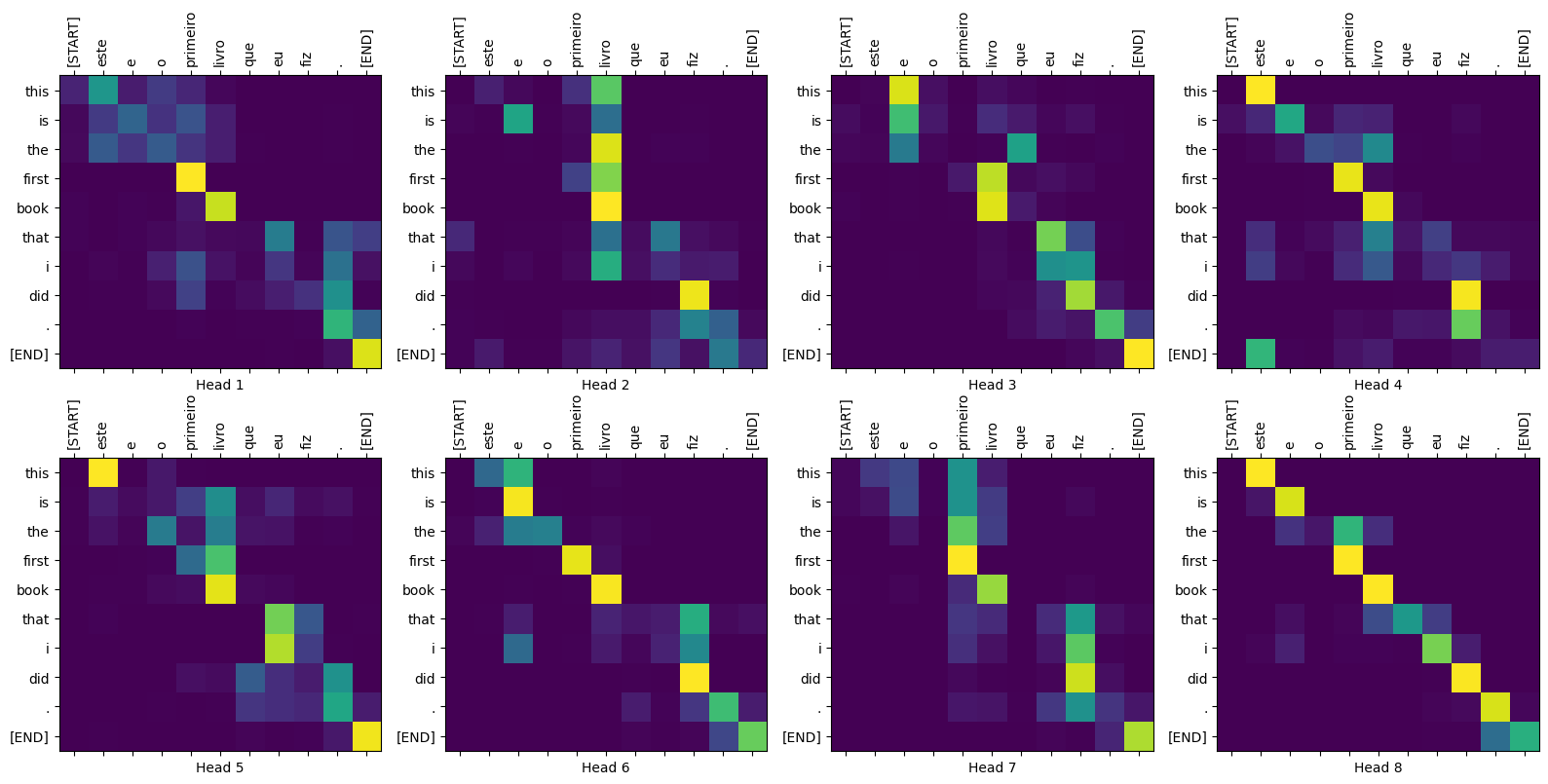
Âm mưu chú ý
Lớp Translator trả về một từ điển bản đồ chú ý mà bạn có thể sử dụng để hình dung hoạt động bên trong của mô hình:
sentence = "este é o primeiro livro que eu fiz."
ground_truth = "this is the first book i've ever done."

translated_text, translated_tokens, attention_weights = translator(
    tf.constant(sentence))
print_translation(sentence, translated_text, ground_truth)
Input:         : este é o primeiro livro que eu fiz.
Prediction     : this is the first book that i did .
Ground truth   : this is the first book i've ever done.
def plot_attention_head(in_tokens, translated_tokens, attention):
  # The plot is of the attention when a token was generated.
  # The model didn't generate `<START>` in the output. Skip it.
  translated_tokens = translated_tokens[1:]

  ax = plt.gca()
  ax.matshow(attention)
  ax.set_xticks(range(len(in_tokens)))
  ax.set_yticks(range(len(translated_tokens)))

  labels = [label.decode('utf-8') for label in in_tokens.numpy()]
  ax.set_xticklabels(
      labels, rotation=90)

  labels = [label.decode('utf-8') for label in translated_tokens.numpy()]
  ax.set_yticklabels(labels)
head = 0
# shape: (batch=1, num_heads, seq_len_q, seq_len_k)
attention_heads = tf.squeeze(
  attention_weights['decoder_layer4_block2'], 0)
attention = attention_heads[head]
attention.shape
TensorShape([10, 11])
in_tokens = tf.convert_to_tensor([sentence])
in_tokens = tokenizers.pt.tokenize(in_tokens).to_tensor()
in_tokens = tokenizers.pt.lookup(in_tokens)[0]
in_tokens
<tf.Tensor: shape=(11,), dtype=string, numpy=
array([b'[START]', b'este', b'e', b'o', b'primeiro', b'livro', b'que',
       b'eu', b'fiz', b'.', b'[END]'], dtype=object)>
translated_tokens
<tf.Tensor: shape=(11,), dtype=string, numpy=
array([b'[START]', b'this', b'is', b'the', b'first', b'book', b'that',
       b'i', b'did', b'.', b'[END]'], dtype=object)>
plot_attention_head(in_tokens, translated_tokens, attention)

def plot_attention_weights(sentence, translated_tokens, attention_heads):
  in_tokens = tf.convert_to_tensor([sentence])
  in_tokens = tokenizers.pt.tokenize(in_tokens).to_tensor()
  in_tokens = tokenizers.pt.lookup(in_tokens)[0]
  in_tokens

  fig = plt.figure(figsize=(16, 8))

  for h, head in enumerate(attention_heads):
    ax = fig.add_subplot(2, 4, h+1)

    plot_attention_head(in_tokens, translated_tokens, head)

    ax.set_xlabel(f'Head {h+1}')

  plt.tight_layout()
  plt.show()
plot_attention_weights(sentence, translated_tokens,
                       attention_weights['decoder_layer4_block2'][0])

Mô hình không ổn đối với các từ không quen thuộc. Cả "triceratops" hoặc "bách khoa toàn thư" đều không có trong tập dữ liệu đầu vào và mô hình gần như học cách chuyển ngữ chúng, ngay cả khi không có từ vựng được chia sẻ:
sentence = "Eu li sobre triceratops na enciclopédia."
ground_truth = "I read about triceratops in the encyclopedia."

translated_text, translated_tokens, attention_weights = translator(
    tf.constant(sentence))
print_translation(sentence, translated_text, ground_truth)

plot_attention_weights(sentence, translated_tokens,
                       attention_weights['decoder_layer4_block2'][0])
Input:         : Eu li sobre triceratops na enciclopédia.
Prediction     : i read about trigatotys in the encyclopedia .
Ground truth   : I read about triceratops in the encyclopedia.

Xuất khẩu
Mô hình suy luận đó đang hoạt động, vì vậy tiếp theo bạn sẽ xuất nó dưới dạng tf.saved_model .
Để làm điều đó, hãy bọc nó trong một lớp con tf.Module khác, lần này với một tf.function trên phương thức __call__ :
class ExportTranslator(tf.Module):
  def __init__(self, translator):
    self.translator = translator

  @tf.function(input_signature=[tf.TensorSpec(shape=[], dtype=tf.string)])
  def __call__(self, sentence):
    (result,
     tokens,
     attention_weights) = self.translator(sentence, max_length=100)

    return result
Trong hàm tf.function ở trên, chỉ câu đầu ra được trả về. Nhờ việc thực thi không nghiêm ngặt trong tf.function mọi giá trị không cần thiết sẽ không bao giờ được tính toán.
translator = ExportTranslator(translator)
Vì mô hình đang giải mã các dự đoán bằng cách sử dụng tf.argmax nên các dự đoán là xác định. Mô hình gốc và một mô hình được tải lại từ SavedModel của nó sẽ đưa ra các dự đoán giống hệt nhau:
translator("este é o primeiro livro que eu fiz.").numpy()
b'this is the first book that i did .'
tf.saved_model.save(translator, export_dir='translator')
2022-02-04 13:19:17.308292: W tensorflow/python/util/util.cc:368] Sets are not currently considered sequences, but this may change in the future, so consider avoiding using them.
WARNING:absl:Found untraced functions such as embedding_4_layer_call_fn, embedding_4_layer_call_and_return_conditional_losses, dropout_37_layer_call_fn, dropout_37_layer_call_and_return_conditional_losses, embedding_5_layer_call_fn while saving (showing 5 of 224). These functions will not be directly callable after loading.
reloaded = tf.saved_model.load('translator')
reloaded("este é o primeiro livro que eu fiz.").numpy()
b'this is the first book that i did .'
Bản tóm tắt
Trong hướng dẫn này, bạn đã học về mã hóa vị trí, sự chú ý nhiều đầu, tầm quan trọng của việc che và cách tạo một máy biến áp.
Hãy thử sử dụng một tập dữ liệu khác để huấn luyện máy biến áp. Bạn cũng có thể tạo biến áp cơ sở hoặc biến áp XL bằng cách thay đổi các siêu tham số ở trên. Bạn cũng có thể sử dụng các lớp được xác định ở đây để tạo BERT và huấn luyện các mô hình hiện đại. Hơn nữa, bạn có thể triển khai tìm kiếm chùm tia để có được những dự đoán tốt hơn.