
|
|
|
 View source on GitHub View source on GitHub
|
|
Setup
First install packages used in this demo.
pip install -q dm-sonnetImports (tf, tfp with adjoint trick, etc)
import numpy as np
import tqdm as tqdm
import sklearn.datasets as skd

# visualization
import matplotlib.pyplot as plt
import seaborn as sns
from scipy.stats import kde

# tf and friends
import tensorflow.compat.v2 as tf
import tensorflow_probability as tfp
import sonnet as snt
tf.enable_v2_behavior()

tfb = tfp.bijectors
tfd = tfp.distributions

def make_grid(xmin, xmax, ymin, ymax, gridlines, pts):
  xpts = np.linspace(xmin, xmax, pts)
  ypts = np.linspace(ymin, ymax, pts)
  xgrid = np.linspace(xmin, xmax, gridlines)
  ygrid = np.linspace(ymin, ymax, gridlines)
  xlines = np.stack([a.ravel() for a in np.meshgrid(xpts, ygrid)])
  ylines = np.stack([a.ravel() for a in np.meshgrid(xgrid, ypts)])
  return np.concatenate([xlines, ylines], 1).T

grid = make_grid(-3, 3, -3, 3, 4, 100)
/usr/local/lib/python3.6/dist-packages/statsmodels/tools/_testing.py:19: FutureWarning: pandas.util.testing is deprecated. Use the functions in the public API at pandas.testing instead.
  import pandas.util.testing as tm
Helper functions for visualization
def plot_density(data, axis):
  x, y = np.squeeze(np.split(data, 2, axis=1))
  levels = np.linspace(0.0, 0.75, 10)
  kwargs = {'levels': levels}
  return sns.kdeplot(x, y, cmap="viridis", shade=True,
                     shade_lowest=True, ax=axis, **kwargs)


def plot_points(data, axis, s=10, color='b', label=''):
  x, y = np.squeeze(np.split(data, 2, axis=1))
  axis.scatter(x, y, c=color, s=s, label=label)


def plot_panel(
    grid, samples, transformed_grid, transformed_samples,
    dataset, axarray, limits=True):
  if len(axarray) != 4:
    raise ValueError('Expected 4 axes for the panel')
  ax1, ax2, ax3, ax4 = axarray
  plot_points(data=grid, axis=ax1, s=20, color='black', label='grid')
  plot_points(samples, ax1, s=30, color='blue', label='samples')
  plot_points(transformed_grid, ax2, s=20, color='black', label='ode(grid)')
  plot_points(transformed_samples, ax2, s=30, color='blue', label='ode(samples)')
  ax3 = plot_density(transformed_samples, ax3)
  ax4 = plot_density(dataset, ax4)
  if limits:
    set_limits([ax1], -3.0, 3.0, -3.0, 3.0)
    set_limits([ax2], -2.0, 3.0, -2.0, 3.0)
    set_limits([ax3, ax4], -1.5, 2.5, -0.75, 1.25)


def set_limits(axes, min_x, max_x, min_y, max_y):
  if isinstance(axes, list):
    for axis in axes:
      set_limits(axis, min_x, max_x, min_y, max_y)
  else:
    axes.set_xlim(min_x, max_x)
    axes.set_ylim(min_y, max_y)
FFJORD bijector
In this colab we demonstrate FFJORD bijector, originally proposed in the paper by Grathwohl, Will, et al. arxiv link.
In the nutshell the idea behind such approach is to establish a correspondence between a known base distribution and the data distribution.
To establish this connection, we need to
- Define a bijective map \(\mathcal{T}_{\theta}:\mathbf{x} \rightarrow \mathbf{y}\), \(\mathcal{T}_{\theta}^{1}:\mathbf{y} \rightarrow \mathbf{x}\) between the space \(\mathcal{Y}\) on which base distribution is defined and space \(\mathcal{X}\) of the data domain.
- Efficiently keep track of the deformations we perform to transfer the notion of probability onto \(\mathcal{X}\).
The second condition is formalized in the following expression for probability distribution defined on \(\mathcal{X}\):
\[ \log p_{\mathbf{x} }(\mathbf{x})=\log p_{\mathbf{y} }(\mathbf{y})-\log \operatorname{det}\left|\frac{\partial \mathcal{T}_{\theta}(\mathbf{y})}{\partial \mathbf{y} }\right| \]
FFJORD bijector accomplishes this by defining a transformation
\[ \mathcal{T_{\theta} }: \mathbf{x} = \mathbf{z}(t_{0}) \rightarrow \mathbf{y} = \mathbf{z}(t_{1}) \quad : \quad \frac{d \mathbf{z} }{dt} = \mathbf{f}(t, \mathbf{z}, \theta) \]
This transformation is invertible, as long as function \(\mathbf{f}\) describing the evolution of the state \(\mathbf{z}\) is well behaved and the log_det_jacobian can be calculated by integrating the following expression.
\[ \log \operatorname{det}\left|\frac{\partial \mathcal{T}_{\theta}(\mathbf{y})}{\partial \mathbf{y} }\right| = -\int_{t_{0} }^{t_{1} } \operatorname{Tr}\left(\frac{\partial \mathbf{f}(t, \mathbf{z}, \theta)}{\partial \mathbf{z}(t)}\right) d t \]
In this demo we will train a FFJORD bijector to warp a gaussian distribution onto the distribution defined by moons dataset. This will be done in 3 steps:
- Define base distribution
- Define FFJORD bijector
- Minimize exact log-likelihood of the dataset
First, we load the data
Dataset
DATASET_SIZE = 1024 * 8
BATCH_SIZE = 256
SAMPLE_SIZE = DATASET_SIZE
moons = skd.make_moons(n_samples=DATASET_SIZE, noise=.06)[0]
moons_ds = tf.data.Dataset.from_tensor_slices(moons.astype(np.float32))
moons_ds = moons_ds.prefetch(tf.data.experimental.AUTOTUNE)
moons_ds = moons_ds.cache()
moons_ds = moons_ds.shuffle(DATASET_SIZE)
moons_ds = moons_ds.batch(BATCH_SIZE)
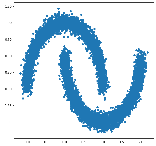
plt.figure(figsize=[8, 8])
plt.scatter(moons[:, 0], moons[:, 1])
plt.show()
Next, we instantiate a base distribution
base_loc = np.array([0.0, 0.0]).astype(np.float32)
base_sigma = np.array([0.8, 0.8]).astype(np.float32)
base_distribution = tfd.MultivariateNormalDiag(base_loc, base_sigma)
We use a multi-layer perceptron to model state_derivative_fn.
While not necessary for this dataset, it is often benefitial to make state_derivative_fn dependent on time. Here we achieve this by concatenating t to inputs of our network.
class MLP_ODE(snt.Module):
  """Multi-layer NN ode_fn."""
  def __init__(self, num_hidden, num_layers, num_output, name='mlp_ode'):
    super(MLP_ODE, self).__init__(name=name)
    self._num_hidden = num_hidden
    self._num_output = num_output
    self._num_layers = num_layers
    self._modules = []
    for _ in range(self._num_layers - 1):
      self._modules.append(snt.Linear(self._num_hidden))
      self._modules.append(tf.math.tanh)
    self._modules.append(snt.Linear(self._num_output))
    self._model = snt.Sequential(self._modules)

  def __call__(self, t, inputs):
    inputs = tf.concat([tf.broadcast_to(t, inputs.shape), inputs], -1)
    return self._model(inputs)
Model and training parameters
LR = 1e-2
NUM_EPOCHS = 80
STACKED_FFJORDS = 4
NUM_HIDDEN = 8
NUM_LAYERS = 3
NUM_OUTPUT = 2
Now we construct a stack of FFJORD bijectors. Each bijector is provided with ode_solve_fn and trace_augmentation_fn and it's own state_derivative_fn model, so that they represent a sequence of different transformations.
Building bijector
solver = tfp.math.ode.DormandPrince(atol=1e-5)
ode_solve_fn = solver.solve
trace_augmentation_fn = tfb.ffjord.trace_jacobian_exact

bijectors = []
for _ in range(STACKED_FFJORDS):
  mlp_model = MLP_ODE(NUM_HIDDEN, NUM_LAYERS, NUM_OUTPUT)
  next_ffjord = tfb.FFJORD(
      state_time_derivative_fn=mlp_model,ode_solve_fn=ode_solve_fn,
      trace_augmentation_fn=trace_augmentation_fn)
  bijectors.append(next_ffjord)

stacked_ffjord = tfb.Chain(bijectors[::-1])
Now we can use TransformedDistribution which is the result of warping base_distribution with stacked_ffjord bijector.
transformed_distribution = tfd.TransformedDistribution(
    distribution=base_distribution, bijector=stacked_ffjord)
Now we define our training procedure. We simply minimize negative log-likelihood of the data.
Training
@tf.function
def train_step(optimizer, target_sample):
  with tf.GradientTape() as tape:
    loss = -tf.reduce_mean(transformed_distribution.log_prob(target_sample))
  variables = tape.watched_variables()
  gradients = tape.gradient(loss, variables)
  optimizer.apply(gradients, variables)
  return loss
Samples
@tf.function
def get_samples():
  base_distribution_samples = base_distribution.sample(SAMPLE_SIZE)
  transformed_samples = transformed_distribution.sample(SAMPLE_SIZE)
  return base_distribution_samples, transformed_samples


@tf.function
def get_transformed_grid():
  transformed_grid = stacked_ffjord.forward(grid)
  return transformed_grid
Plot samples from base and transformed distributions.
evaluation_samples = []
base_samples, transformed_samples = get_samples()
transformed_grid = get_transformed_grid()
evaluation_samples.append((base_samples, transformed_samples, transformed_grid))
WARNING:tensorflow:From /usr/local/lib/python3.6/dist-packages/tensorflow/python/ops/resource_variable_ops.py:1817: calling BaseResourceVariable.__init__ (from tensorflow.python.ops.resource_variable_ops) with constraint is deprecated and will be removed in a future version.
Instructions for updating:
If using Keras pass *_constraint arguments to layers.
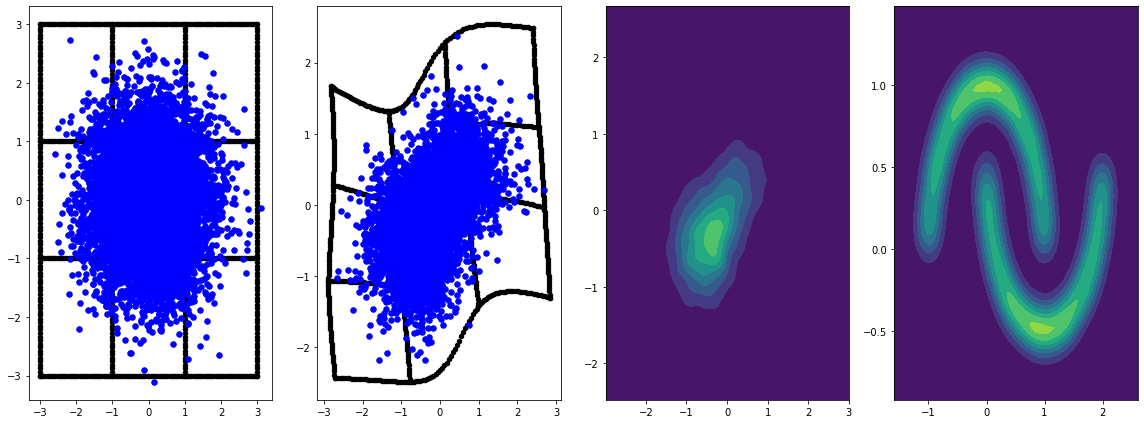
panel_id = 0
panel_data = evaluation_samples[panel_id]
fig, axarray = plt.subplots(
  1, 4, figsize=(16, 6))
plot_panel(
    grid, panel_data[0], panel_data[2], panel_data[1], moons, axarray, False)
plt.tight_layout()
learning_rate = tf.Variable(LR, trainable=False)
optimizer = snt.optimizers.Adam(learning_rate)

for epoch in tqdm.trange(NUM_EPOCHS // 2):
  base_samples, transformed_samples = get_samples()
  transformed_grid = get_transformed_grid()
  evaluation_samples.append(
      (base_samples, transformed_samples, transformed_grid))
  for batch in moons_ds:
    _ = train_step(optimizer, batch)
0%|          | 0/40 [00:00<?, ?it/s]
WARNING:tensorflow:From /usr/local/lib/python3.6/dist-packages/tensorflow_probability/python/math/ode/base.py:350: calling while_loop_v2 (from tensorflow.python.ops.control_flow_ops) with back_prop=False is deprecated and will be removed in a future version.
Instructions for updating:
back_prop=False is deprecated. Consider using tf.stop_gradient instead.
Instead of:
results = tf.while_loop(c, b, vars, back_prop=False)
Use:
results = tf.nest.map_structure(tf.stop_gradient, tf.while_loop(c, b, vars))
100%|██████████| 40/40 [07:00<00:00, 10.52s/it]
panel_id = -1
panel_data = evaluation_samples[panel_id]
fig, axarray = plt.subplots(
  1, 4, figsize=(16, 6))
plot_panel(grid, panel_data[0], panel_data[2], panel_data[1], moons, axarray)
plt.tight_layout()
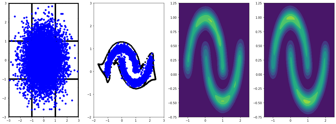
Training it for longer with learning rate results in further improvements.
Not convered in this example, FFJORD bijector supports hutchinson's stochastic trace estimation. The particular estimator can be provided via trace_augmentation_fn. Similarly alternative integrators can be used by defining custom ode_solve_fn.