TF Lattice Canned Estimators

Warning: Estimators are not recommended for new code. Estimators run v1. Session-style code which is more difficult to write correctly, and can behave unexpectedly, especially when combined with TF 2 code. Estimators do fall under our compatibility guarantees, but will receive no fixes other than security vulnerabilities. See the migration guide for details.

Overview

Canned estimators are quick and easy ways to train TFL models for typical use cases. This guide outlines the steps needed to create a TFL canned estimator.

Setup

Installing TF Lattice package:

pip install tensorflow-lattice

Importing required packages:

import tensorflow as tf

import copy
import logging
import numpy as np
import pandas as pd
import sys
import tensorflow_lattice as tfl
from tensorflow import feature_column as fc
logging.disable(sys.maxsize)

2023-09-29 11:04:38.659937: E tensorflow/compiler/xla/stream_executor/cuda/cuda_dnn.cc:9342] Unable to register cuDNN factory: Attempting to register factory for plugin cuDNN when one has already been registered
2023-09-29 11:04:38.659988: E tensorflow/compiler/xla/stream_executor/cuda/cuda_fft.cc:609] Unable to register cuFFT factory: Attempting to register factory for plugin cuFFT when one has already been registered
2023-09-29 11:04:38.660024: E tensorflow/compiler/xla/stream_executor/cuda/cuda_blas.cc:1518] Unable to register cuBLAS factory: Attempting to register factory for plugin cuBLAS when one has already been registered

Downloading the UCI Statlog (Heart) dataset:

csv_file = tf.keras.utils.get_file(
    'heart.csv', 'http://storage.googleapis.com/download.tensorflow.org/data/heart.csv')
df = pd.read_csv(csv_file)
target = df.pop('target')
train_size = int(len(df) * 0.8)
train_x = df[:train_size]
train_y = target[:train_size]
test_x = df[train_size:]
test_y = target[train_size:]
df.head()

Downloading data from http://storage.googleapis.com/download.tensorflow.org/data/heart.csv
13273/13273 [==============================] - 0s 0us/step

Setting the default values used for training in this guide:

LEARNING_RATE = 0.01
BATCH_SIZE = 128
NUM_EPOCHS = 500
PREFITTING_NUM_EPOCHS = 10

Feature Columns

As for any other TF estimator, data needs to be passed to the estimator, which is typically via an input_fn and parsed using FeatureColumns.

# Feature columns.
# - age
# - sex
# - cp        chest pain type (4 values)
# - trestbps  resting blood pressure
# - chol      serum cholestoral in mg/dl
# - fbs       fasting blood sugar > 120 mg/dl
# - restecg   resting electrocardiographic results (values 0,1,2)
# - thalach   maximum heart rate achieved
# - exang     exercise induced angina
# - oldpeak   ST depression induced by exercise relative to rest
# - slope     the slope of the peak exercise ST segment
# - ca        number of major vessels (0-3) colored by flourosopy
# - thal      3 = normal; 6 = fixed defect; 7 = reversable defect
feature_columns = [
    fc.numeric_column('age', default_value=-1),
    fc.categorical_column_with_vocabulary_list('sex', [0, 1]),
    fc.numeric_column('cp'),
    fc.numeric_column('trestbps', default_value=-1),
    fc.numeric_column('chol'),
    fc.categorical_column_with_vocabulary_list('fbs', [0, 1]),
    fc.categorical_column_with_vocabulary_list('restecg', [0, 1, 2]),
    fc.numeric_column('thalach'),
    fc.categorical_column_with_vocabulary_list('exang', [0, 1]),
    fc.numeric_column('oldpeak'),
    fc.categorical_column_with_vocabulary_list('slope', [0, 1, 2]),
    fc.numeric_column('ca'),
    fc.categorical_column_with_vocabulary_list(
        'thal', ['normal', 'fixed', 'reversible']),
]

TFL canned estimators use the type of the feature column to decide what type of calibration layer to use. We use a tfl.layers.PWLCalibration layer for numeric feature columns and a tfl.layers.CategoricalCalibration layer for categorical feature columns.

Note that categorical feature columns are not wrapped by an embedding feature column. They are directly fed into the estimator.

Creating input_fn

As for any other estimator, you can use an input_fn to feed data to the model for training and evaluation. TFL estimators can automatically calculate quantiles of the features and use them as input keypoints for the PWL calibration layer. To do so, they require passing a feature_analysis_input_fn, which is similar to the training input_fn but with a single epoch or a subsample of the data.

train_input_fn = tf.compat.v1.estimator.inputs.pandas_input_fn(
    x=train_x,
    y=train_y,
    shuffle=False,
    batch_size=BATCH_SIZE,
    num_epochs=NUM_EPOCHS,
    num_threads=1)

# feature_analysis_input_fn is used to collect statistics about the input.
feature_analysis_input_fn = tf.compat.v1.estimator.inputs.pandas_input_fn(
    x=train_x,
    y=train_y,
    shuffle=False,
    batch_size=BATCH_SIZE,
    # Note that we only need one pass over the data.
    num_epochs=1,
    num_threads=1)

test_input_fn = tf.compat.v1.estimator.inputs.pandas_input_fn(
    x=test_x,
    y=test_y,
    shuffle=False,
    batch_size=BATCH_SIZE,
    num_epochs=1,
    num_threads=1)

# Serving input fn is used to create saved models.
serving_input_fn = (
    tf.estimator.export.build_parsing_serving_input_receiver_fn(
        feature_spec=fc.make_parse_example_spec(feature_columns)))

Feature Configs

Feature calibration and per-feature configurations are set using tfl.configs.FeatureConfig. Feature configurations include monotonicity constraints, per-feature regularization (see tfl.configs.RegularizerConfig), and lattice sizes for lattice models.

If no configuration is defined for an input feature, the default configuration in tfl.config.FeatureConfig is used.

# Feature configs are used to specify how each feature is calibrated and used.
feature_configs = [
    tfl.configs.FeatureConfig(
        name='age',
        lattice_size=3,
        # By default, input keypoints of pwl are quantiles of the feature.
        pwl_calibration_num_keypoints=5,
        monotonicity='increasing',
        pwl_calibration_clip_max=100,
        # Per feature regularization.
        regularizer_configs=[
            tfl.configs.RegularizerConfig(name='calib_wrinkle', l2=0.1),
        ],
    ),
    tfl.configs.FeatureConfig(
        name='cp',
        pwl_calibration_num_keypoints=4,
        # Keypoints can be uniformly spaced.
        pwl_calibration_input_keypoints='uniform',
        monotonicity='increasing',
    ),
    tfl.configs.FeatureConfig(
        name='chol',
        # Explicit input keypoint initialization.
        pwl_calibration_input_keypoints=[126.0, 210.0, 247.0, 286.0, 564.0],
        monotonicity='increasing',
        # Calibration can be forced to span the full output range by clamping.
        pwl_calibration_clamp_min=True,
        pwl_calibration_clamp_max=True,
        # Per feature regularization.
        regularizer_configs=[
            tfl.configs.RegularizerConfig(name='calib_hessian', l2=1e-4),
        ],
    ),
    tfl.configs.FeatureConfig(
        name='fbs',
        # Partial monotonicity: output(0) <= output(1)
        monotonicity=[(0, 1)],
    ),
    tfl.configs.FeatureConfig(
        name='trestbps',
        pwl_calibration_num_keypoints=5,
        monotonicity='decreasing',
    ),
    tfl.configs.FeatureConfig(
        name='thalach',
        pwl_calibration_num_keypoints=5,
        monotonicity='decreasing',
    ),
    tfl.configs.FeatureConfig(
        name='restecg',
        # Partial monotonicity: output(0) <= output(1), output(0) <= output(2)
        monotonicity=[(0, 1), (0, 2)],
    ),
    tfl.configs.FeatureConfig(
        name='exang',
        # Partial monotonicity: output(0) <= output(1)
        monotonicity=[(0, 1)],
    ),
    tfl.configs.FeatureConfig(
        name='oldpeak',
        pwl_calibration_num_keypoints=5,
        monotonicity='increasing',
    ),
    tfl.configs.FeatureConfig(
        name='slope',
        # Partial monotonicity: output(0) <= output(1), output(1) <= output(2)
        monotonicity=[(0, 1), (1, 2)],
    ),
    tfl.configs.FeatureConfig(
        name='ca',
        pwl_calibration_num_keypoints=4,
        monotonicity='increasing',
    ),
    tfl.configs.FeatureConfig(
        name='thal',
        # Partial monotonicity:
        # output(normal) <= output(fixed)
        # output(normal) <= output(reversible)        
        monotonicity=[('normal', 'fixed'), ('normal', 'reversible')],
    ),
]

Calibrated Linear Model

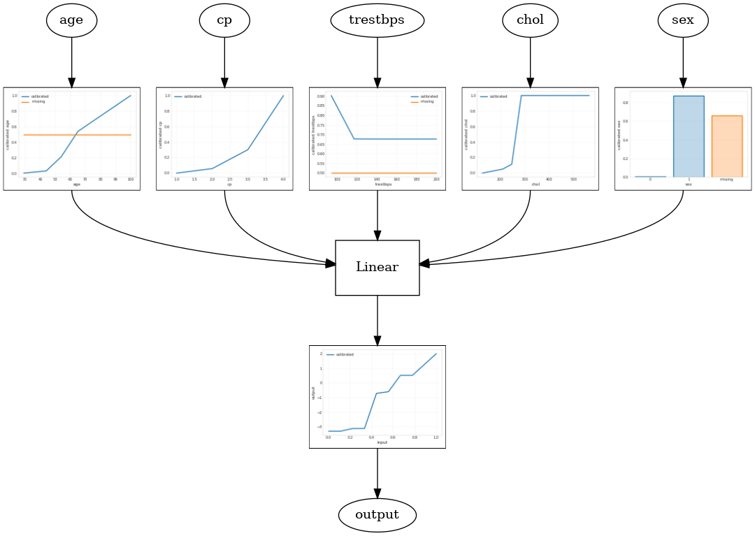
To construct a TFL canned estimator, construct a model configuration from tfl.configs. A calibrated linear model is constructed using tfl.configs.CalibratedLinearConfig. It applies piecewise-linear and categorical calibration on the input features, followed by a linear combination and an optional output piecewise-linear calibration. When using output calibration or when output bounds are specified, the linear layer will apply weighted averaging on calibrated inputs.

This example creates a calibrated linear model on the first 5 features. We use tfl.visualization to plot the model graph with the calibrator plots.

# Model config defines the model structure for the estimator.
model_config = tfl.configs.CalibratedLinearConfig(
    feature_configs=feature_configs,
    use_bias=True,
    output_calibration=True,
    regularizer_configs=[
        # Regularizer for the output calibrator.
        tfl.configs.RegularizerConfig(name='output_calib_hessian', l2=1e-4),
    ])
# A CannedClassifier is constructed from the given model config.
estimator = tfl.estimators.CannedClassifier(
    feature_columns=feature_columns[:5],
    model_config=model_config,
    feature_analysis_input_fn=feature_analysis_input_fn,
    optimizer=tf.keras.optimizers.legacy.Adam(LEARNING_RATE),
    config=tf.estimator.RunConfig(tf_random_seed=42))
estimator.train(input_fn=train_input_fn)
results = estimator.evaluate(input_fn=test_input_fn)
print('Calibrated linear test AUC: {}'.format(results['auc']))
saved_model_path = estimator.export_saved_model(estimator.model_dir,
                                                serving_input_fn)
model_graph = tfl.estimators.get_model_graph(saved_model_path)
tfl.visualization.draw_model_graph(model_graph)

2023-09-29 11:04:41.569210: E tensorflow/compiler/xla/stream_executor/cuda/cuda_driver.cc:268] failed call to cuInit: CUDA_ERROR_NO_DEVICE: no CUDA-capable device is detected
Calibrated linear test AUC: 0.8370927572250366

png

Calibrated Lattice Model

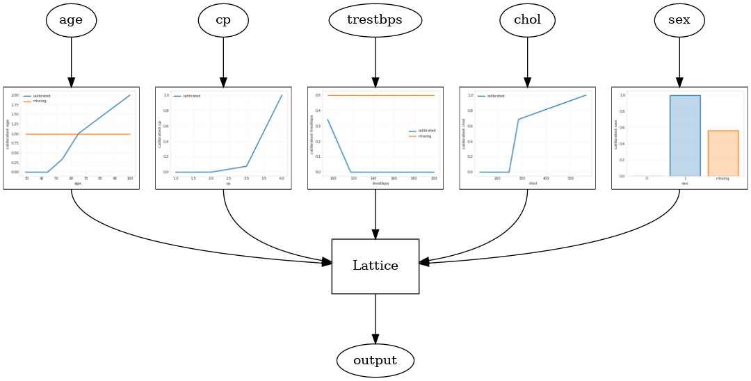
A calibrated lattice model is constructed using tfl.configs.CalibratedLatticeConfig. A calibrated lattice model applies piecewise-linear and categorical calibration on the input features, followed by a lattice model and an optional output piecewise-linear calibration.

This example creates a calibrated lattice model on the first 5 features.

# This is calibrated lattice model: Inputs are calibrated, then combined
# non-linearly using a lattice layer.
model_config = tfl.configs.CalibratedLatticeConfig(
    feature_configs=feature_configs,
    regularizer_configs=[
        # Torsion regularizer applied to the lattice to make it more linear.
        tfl.configs.RegularizerConfig(name='torsion', l2=1e-4),
        # Globally defined calibration regularizer is applied to all features.
        tfl.configs.RegularizerConfig(name='calib_hessian', l2=1e-4),
    ])
# A CannedClassifier is constructed from the given model config.
estimator = tfl.estimators.CannedClassifier(
    feature_columns=feature_columns[:5],
    model_config=model_config,
    feature_analysis_input_fn=feature_analysis_input_fn,
    optimizer=tf.keras.optimizers.legacy.Adam(LEARNING_RATE),
    config=tf.estimator.RunConfig(tf_random_seed=42))
estimator.train(input_fn=train_input_fn)
results = estimator.evaluate(input_fn=test_input_fn)
print('Calibrated lattice test AUC: {}'.format(results['auc']))
saved_model_path = estimator.export_saved_model(estimator.model_dir,
                                                serving_input_fn)
model_graph = tfl.estimators.get_model_graph(saved_model_path)
tfl.visualization.draw_model_graph(model_graph)

Calibrated lattice test AUC: 0.8427318930625916

png

Calibrated Lattice Ensemble

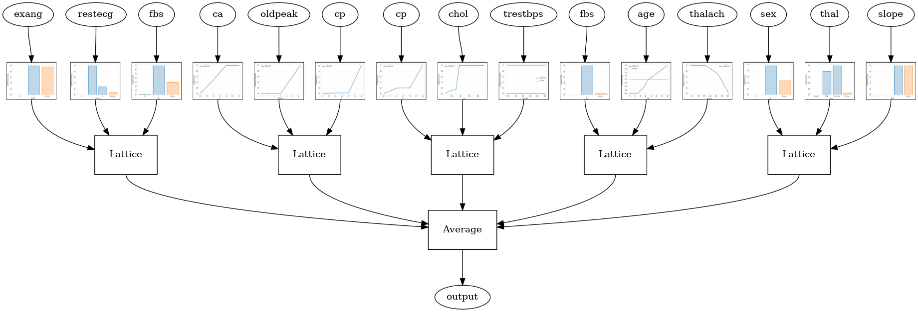
When the number of features is large, you can use an ensemble model, which creates multiple smaller lattices for subsets of the features and averages their output instead of creating just a single huge lattice. Ensemble lattice models are constructed using tfl.configs.CalibratedLatticeEnsembleConfig. A calibrated lattice ensemble model applies piecewise-linear and categorical calibration on the input feature, followed by an ensemble of lattice models and an optional output piecewise-linear calibration.

Random Lattice Ensemble

The following model config uses a random subset of features for each lattice.

# This is random lattice ensemble model with separate calibration:
# model output is the average output of separately calibrated lattices.
model_config = tfl.configs.CalibratedLatticeEnsembleConfig(
    feature_configs=feature_configs,
    num_lattices=5,
    lattice_rank=3)
# A CannedClassifier is constructed from the given model config.
estimator = tfl.estimators.CannedClassifier(
    feature_columns=feature_columns,
    model_config=model_config,
    feature_analysis_input_fn=feature_analysis_input_fn,
    optimizer=tf.keras.optimizers.legacy.Adam(LEARNING_RATE),
    config=tf.estimator.RunConfig(tf_random_seed=42))
estimator.train(input_fn=train_input_fn)
results = estimator.evaluate(input_fn=test_input_fn)
print('Random ensemble test AUC: {}'.format(results['auc']))
saved_model_path = estimator.export_saved_model(estimator.model_dir,
                                                serving_input_fn)
model_graph = tfl.estimators.get_model_graph(saved_model_path)
tfl.visualization.draw_model_graph(model_graph, calibrator_dpi=15)

Random ensemble test AUC: 0.9035087823867798

png

RTL Layer Random Lattice Ensemble

The following model config uses a tfl.layers.RTL layer that uses a random subset of features for each lattice. We note that tfl.layers.RTL only supports monotonicity constraints and must have the same lattice size for all features and no per-feature regularization. Note that using a tfl.layers.RTL layer lets you scale to much larger ensembles than using separate tfl.layers.Lattice instances.

# Make sure our feature configs have the same lattice size, no per-feature
# regularization, and only monotonicity constraints.
rtl_layer_feature_configs = copy.deepcopy(feature_configs)
for feature_config in rtl_layer_feature_configs:
  feature_config.lattice_size = 2
  feature_config.unimodality = 'none'
  feature_config.reflects_trust_in = None
  feature_config.dominates = None
  feature_config.regularizer_configs = None
# This is RTL layer ensemble model with separate calibration:
# model output is the average output of separately calibrated lattices.
model_config = tfl.configs.CalibratedLatticeEnsembleConfig(
    lattices='rtl_layer',
    feature_configs=rtl_layer_feature_configs,
    num_lattices=5,
    lattice_rank=3)
# A CannedClassifier is constructed from the given model config.
estimator = tfl.estimators.CannedClassifier(
    feature_columns=feature_columns,
    model_config=model_config,
    feature_analysis_input_fn=feature_analysis_input_fn,
    optimizer=tf.keras.optimizers.legacy.Adam(LEARNING_RATE),
    config=tf.estimator.RunConfig(tf_random_seed=42))
estimator.train(input_fn=train_input_fn)
results = estimator.evaluate(input_fn=test_input_fn)
print('Random ensemble test AUC: {}'.format(results['auc']))
saved_model_path = estimator.export_saved_model(estimator.model_dir,
                                                serving_input_fn)
model_graph = tfl.estimators.get_model_graph(saved_model_path)
tfl.visualization.draw_model_graph(model_graph, calibrator_dpi=15)

Random ensemble test AUC: 0.891603946685791

png

Crystals Lattice Ensemble

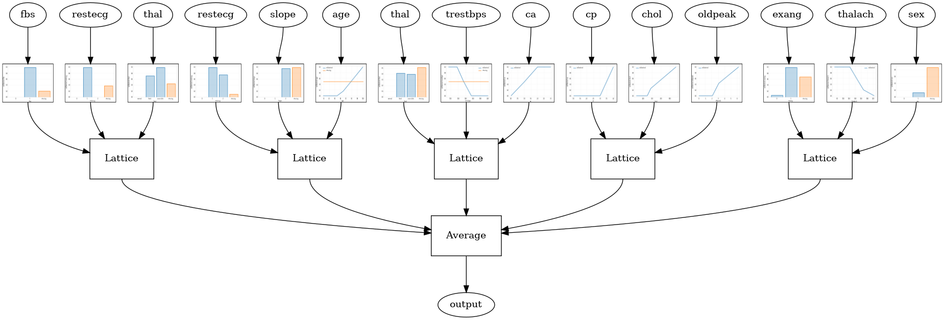
TFL also provides a heuristic feature arrangement algorithm, called Crystals. The Crystals algorithm first trains a prefitting model that estimates pairwise feature interactions. It then arranges the final ensemble such that features with more non-linear interactions are in the same lattices.

For Crystals models, you will also need to provide a prefitting_input_fn that is used to train the prefitting model, as described above. The prefitting model does not need to be fully trained, so a few epochs should be enough.

prefitting_input_fn = tf.compat.v1.estimator.inputs.pandas_input_fn(
    x=train_x,
    y=train_y,
    shuffle=False,
    batch_size=BATCH_SIZE,
    num_epochs=PREFITTING_NUM_EPOCHS,
    num_threads=1)

You can then create a Crystal model by setting lattice='crystals' in the model config.

# This is Crystals ensemble model with separate calibration: model output is
# the average output of separately calibrated lattices.
model_config = tfl.configs.CalibratedLatticeEnsembleConfig(
    feature_configs=feature_configs,
    lattices='crystals',
    num_lattices=5,
    lattice_rank=3)
# A CannedClassifier is constructed from the given model config.
estimator = tfl.estimators.CannedClassifier(
    feature_columns=feature_columns,
    model_config=model_config,
    feature_analysis_input_fn=feature_analysis_input_fn,
    # prefitting_input_fn is required to train the prefitting model.
    prefitting_input_fn=prefitting_input_fn,
    optimizer=tf.keras.optimizers.legacy.Adam(LEARNING_RATE),
    prefitting_optimizer=tf.keras.optimizers.legacy.Adam(LEARNING_RATE),
    config=tf.estimator.RunConfig(tf_random_seed=42))
estimator.train(input_fn=train_input_fn)
results = estimator.evaluate(input_fn=test_input_fn)
print('Crystals ensemble test AUC: {}'.format(results['auc']))
saved_model_path = estimator.export_saved_model(estimator.model_dir,
                                                serving_input_fn)
model_graph = tfl.estimators.get_model_graph(saved_model_path)
tfl.visualization.draw_model_graph(model_graph, calibrator_dpi=15)

Crystals ensemble test AUC: 0.9078947305679321

png

You can plot feature calibrators with more details using the tfl.visualization module.

_ = tfl.visualization.plot_feature_calibrator(model_graph, "age")
_ = tfl.visualization.plot_feature_calibrator(model_graph, "restecg")